
Most of the theory is pretty basic and given in the video lecture. The object of the test is to plot the deadweight pressures (reference) against those reported by the gauges. Scroll down for the procedure; the data spreadsheet for pressure gauge testing is here. The procedure covers both what was done in the lab physically and also has a specific section for the video procedure. The data collection and analysis procedure for both is the same, but the way the tester is rigged is different.
Other Resources:
- Chauvenet’s Criterion (video overview)
- Fluid Power Systems: An Overview and Design Example
- An Overview of Tapered Pipe Threads, and Their Application at Vulcan, which is how the gauges are held to the pressure gauge tester.
- Blessed are the Merciful: What students ask me when they’re under pressure.
Introduction:
Most pressure-measuring devices measure pressure differences, not absolute pressure. For example, the common Bourdon-type pressure gauge indicates only the difference between the absolute pressure in the fluid to which it is connected and the pressure of the atmosphere around the gauge. This type of pressure measurement is therefore known as “gauge pressure.”
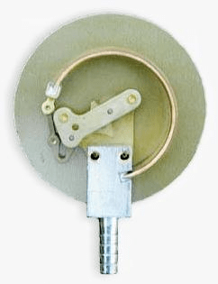
The Bourdon-type gauge (see right, from Wikipedia) consists of a tube having an elliptical cross-section bent into a circular arc. When atmospheric pressure (i.e. zero gauge pressure) prevails in the gauge, the tube is undeflected (as fabricated) with the gauge pointer positioned to read zero pressure. When pressure is applied to the gauge, the curved tube tends to straighten, thereby moving the pointer through the linkage mechanism. The gauge pressure can be indicated at the tip of the pointer. After the gauge is developed and initially calibrated, the gauge pressures will be displayed in print on the face of the gauge. However, manufacturing techniques and/or quality control does not assure that each gauge manufactured performs similarly.
The Bourdon gauge is calibrated using a dead-weight tester. Ideally, the gauge reading indicated by the pointer should correspond to the hydrostatic pressure applied by the dead-weight tester. Inexpensive Bourdon gauges (like those purchased from the local hardware store) have not been calibrated using a dead-weight tester. In contrast, high quality gauges measuring pressures that are monitored in central control rooms (e.g. at a TVA nuclear power plant) must be calibrated and at considerable expense, possibly many times during their lifetime. The Bourdon pressure gauge is used in a wide range of applications, with accuracy and linearity depending on the quality of the gauge.
Theory/Procedures:
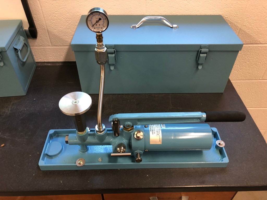
Three (3) Ashcroft dead-weight testers will be used to concurrently calibrate three Bourdon gauges. The three Ashcroft testers as set up in the lab are shown below.

The gauges to be tested will be in increasing maximum pressure from left to right. The lowest pressure gauge on the right is shown below.
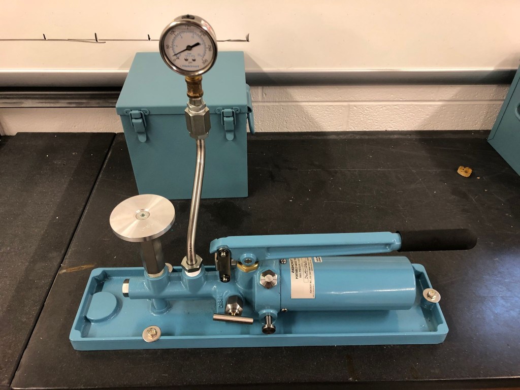
The second one in the middle is shown below.
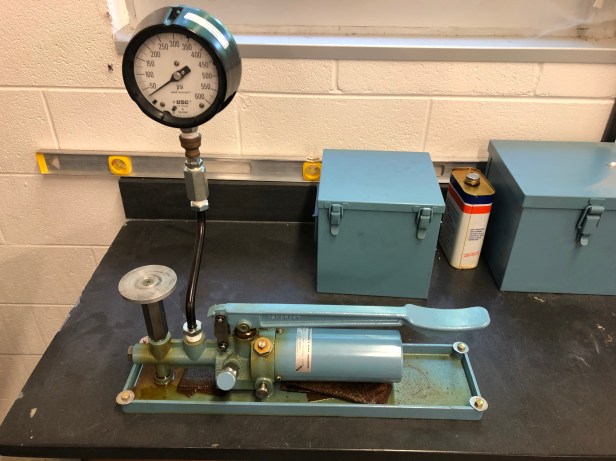
The one on the left is shown below.
Two different piston-cylinders are available, providing two pressure ranges:
- Low (L), 15-200 psig; and
- High (H) 75-1000 psig
It is very important, when you are loading a pressure gauge tester, to make sure that you are using the correct pressure (L or H) stamped on the weight. The right and middle pressure gauge testers are set up for low (L) range and the one on the left is set up for the high (H) range. The chamber and cylinder of the tester should be filled with clean oil and primed to remove air from within the system.
Each of the testers is operated as follows:
- The release valve is closed.
- A weight (or more often combination of weights) is loaded onto the deck. The deck itself has a pressure associated with it. The reference pressure is the sum of the pressures of the weights. The sequence of the pressures desired is shown in the sample data spreadsheet. It’s easy to lose track when switching weights, be careful.
- The handle is pumped until the weight stack floats between the top and bottom stops of the piston. Especially with the low pressures, this may take some “fiddling.” The easiest way to make sure that the weight stack is really floating is to “bounce” the stack up and down, making sure it hits neither the top nor the bottom stop. It’s possible sometimes to use the displacement knob on the back of the tester for fine adjustments, but given the amount of air usually in these testers generally this isn’t effective.
- Record both the reference pressure of the weight stack and the reading on the gauge.
- Load the stack to the next pressure shown on the data spreadsheet and repeat Steps 2-4.
- After reaching the maximum pressure, release the pressure, making sure it’s at zero. Remove the weights from the stack.
When you’re finished with one tester, move on to the next one. When you’ve completed all three testers, you are done. Each group of students should develop at least three (3) complete sets of data; all of the sets are to be shared with the rest of the group, which can be done in Canvas.
Video Data Collection
If you are able to come to the lab, you will collect the data physically; however, in the event that you cannot you will need to collect the data from the video. The video was recorded when the setup was a little different, specifically only one high-pressure setup was used for all three gauges. The video explains how the gauges are tested and the valves manipulated to obtain the result. Eliminating valve manipulation (and thus having more than one machine available at a time) was a major reason the additional pressure gauge testers were purchased. They are essentially the same as the original one shown in the video.
The data spreadsheet has a separate sheet for recording the video data. The data spreadsheet for the video data has the other two sets of data you’ll need to perform Chauvenet’s Criterion. You also need to plot the deadweight vs. gauge pressures for all three gauges and to analyze this data.
Results:
- Develop tables comparing the gage pressure indicated on the gage (Pindicated) versus the dead-weight tester applied pressure (Pactual) for each gage; this should include data obtained by all groups. We recommend using the sample data spreadsheet that accompanies this lab.
- Analyze each data point (deadweight pressure and specific tester) and gauge reading in a given data point using Chauvenet’s criterion. Information on Chauvenet’s Criterion appears at the end of the handout. How many gauge readings you have for each data point will vary depending upon the way the experiment is run. In any case, compare each gauge reading to Chauvenet’s Criterion and, if a point is an outlier according to the Criterion, eliminate it from any future averaging.
- With the remaining data, plot the average indicated pressure (y-axis) versus the dead-weight pressure (x-axis.) There should be a separate figure for each of the three gauges tested. The figures should be in the analysis portion of the report.
- Using linear regression, find the best fit line of the data plotted in each figure; be sure to include the equation and R2 value on the plot. The resulting equation should be of the form:
Pindicated = m*Pactual + b (1)
with an “ideal” gauge having m = 1 and b = 0.0 psig.
What to Include in the Report:
- A title sheet (see the Lab Report Layout handout on Blackboard).
- A main body containing the following sections:
- Objective(s) – What was the purpose of the experiment?
- Theory/Procedure – Include your interpretation of this section using the information provided in the handout.
- Observed Data – Put the data into tabular form, with units, using the sample lab spreadsheet. Be sure to place an appropriate title caption above the table (see Lab Report Guidelines handout on Blackboard) and include a few sentences to orient the reader.
- Results/Discussion – Present and discuss the results of your calibration efforts. Provide a separate, standard Cartesian (y vs. x) figure for each gage, plotting the average Pindicated vs. Pactual. Find the best fit straight line through each data set using linear regression. Show the best fit line with its equation and R2 value on the graph. Be sure to include an appropriate title below each figure (see Lab Report Guidelines handout on UTC Learn). Calculate Chauvenet’s Criterion for each individual measurement; present the results in tabular form.
- Conclusions – What did you learn? Did you accomplish your objectives? Are the gauges accurate? Does the use of the calibration curve compensate for any deficiencies? Can these gauges be used with confidence? Does the use of statistics (i.e. Chauvenet’s Criterion) provide for a better gauge calibration?
- Appendix –Provide a sample calculation for a complete data set from your experimental data.
- References – Include any references cited here.
Chauvenet’s Criterion
Chauvenet’s criterion is used to identify outliers to the data in a statistically consistent fashion. It is done as follows:
- Determine the mean and standard deviation for each true pressure reading; enter these into the table.
- Determine Chauvenet’s “Z” factor from Table 2. This is strictly a function of the number of data points you have.
- A data point is an outlier according to Chauvenet’s Criterion if the following condition is met:
Z < |y-ymean|/σ (2a)
or
Zσ < |y-ymean| (2b)
Where y = y-value of data point in question, ymean = mean value of the data points, and σ = standard deviation of the data points.
- Apply this to the data you have. If a data point a) exceeds the deviation allowed by Chauvenet’s Criterion and b) is the largest deviation, it can be excluded, and the mean computed from the rest of the data points. This mean is then applied to your comparison with the true pressure.
Table 2 Chauvenet’s “Z” Factor
| Number of Data Points | Chauvenet “Z” Factor |
| 3 | 1.38 |
| 4 | 1.54 |
| 5 | 1.65 |
| 6 | 1.73 |
| 7 | 1.80 |
| 8 | 1.87 |
| 9 | 1.91 |
| 10 | 1.96 |
As an example, consider a data point where the deadweight pressure is 100 psig and the gauge returns three different values for three different tests: 84, 94, and 92 psi. The mean of this data is 92 psi and the standard deviation is 7.21 psi. The three data points vary from the mean by the absolute values of 6, 8 and 2 psi respectively. For three data points, Chauvenet’s “Z” factor is 1.38 from the table above. From Equation (2), the maximum deviation permitted by Chauvenet’s Criterion is (7.21)(1.38) = 9.95 psi. As you can see, none of the deviations exceed this, so all of the data points are within the Criterion.
- Since the deviations of the data points are within the maximum deviation allowed by Chauvenet’s Criterion, use all of the data points, take the average, and use that average in your linear regression analysis of the data.
- If a data point falls outside of Chauvenet’s Criterion, throw it out, average the rest, and use that result as your average value for the linear regression.
This example is included in your data spreadsheet.
