Mohr’s Circle Analysis Using Linear Algebra and Numerical Methods

Abstract

Mohr’s Circle-or more generally the stress equilibrium in solids-is a well known method to analyse the stress state of a two- or three-dimensional solid. Most engineers are exposed to its derivation using ordinary algebra, especially as it relates to the determination of principal stresses and invariants for comparison with failure criteria. In this presentation, an approach using linear algebra will be set forth, which is interesting not only from the standpoint of the stress state but from linear algebra considerations, as the problem makes an excellent illustration of linear algebra concepts from a real geometric system. A numerical implementation of the solution using Danilevsky’s Method will be detailed.

Update: the online routine, which was the progression past the FORTRAN routine shown here, is being phased out. You can see this routine in spreadsheet form here, where there is also a link to the updated monograph. Other improvements to this routine are documented here as well.

1. Introduction

The analysis of the stress state of a solid at a given point is a basic part of mechanics of materials.Although such analysis is generally associated with the theory of elasticity, in fact it is based on static equilibrium, and is also valid for the plastic region as well. In this way it is used in non-linear finite element analysis, among other applications. The usual objective of such an analysis is to determine the principal stresses at a point, which in turn can be compared to failure criteria to determine local deformation.In this approach the governing equations will be cast in a linear algebra form and the problem solved in this way, as opposed to other types of solutions given in various textbooks. Doing it in this way can have three results:

1. It allows the abstract concepts of linear algebra to be illustrated well in a physical problem.
2. It allows the physics of the determination of principal stresses to be seen in a different way with the mathematics.
3. It opens up the problem to numerical solution, as opposed to the complicated closed-form solutions usually encountered, of the invariants, principal stresses or direction cosines.

2. Two-Dimensional Analysis

2.1. Eigenvalues, Eigenvectors and Principal Stresses

The simplest way to illustrate this is to use two-dimensional analysis. Even with this simplest case, the algebra can become very difficult very quickly, and the concepts themselves obscured. Consider first the stress state shown in Figure 1, with the notation which will be used in the rest of the article.

The theory behind this figure is described in many mechanics of materials textbooks; for this case the presentation of Jaeger and Cook [4] was used. The element is in static equilibrium along both axes. In order for the summation of moments to be zero,

(1)

The angles are done a little differently than usual; this is to allow an easier transition when three-dimensional analysis is considered. The direction cosines based on these angles are as follows:

(2)

(3)

Now consider the components of the stress vector p on their respective axes. Putting these into matrix form, they are computed as follows:

$latex \left[\begin{array}{cc}
\sigma_{{x}} & \tau_{{\it xy}}\\
\noalign{\medskip}\tau_{{\it xy}} & \sigma_{{y}}
\end{array}\right]\left[\begin{array}{c}
l\\
\noalign{\medskip}m
\end{array}\right]=\left[\begin{array}{c}
p_{{x}}\\
\noalign{\medskip}p_{{y}}
\end{array}\right] $ (4)

which is a classic Ax = b type of problem. At this point there are some things about the matrix in Equation 4 that need to be noted (DeRusso et al. [2]):

1. It is square.
2. It is real and symmetric. Because of these two properties:
   1. The eigenvalues (and thus the principal stresses, as will be shown) are real. Since for two-dimensional space the equations for the principal stresses are quadratic, this is not a “given” from pure algebra alone.
   2. The eigenvectors form an orthogonal set, which is important in the diagonalization process.
3. The sum of the diagonal entries of the matrix, referred to as the trace, is equal to the sum of the values of the eigenvalues. As will be seen, this means that, as we rotate the coordinate axes, the trace remains invariant.

At this point there are two related questions that need to be asked. The first is whether static equilibrium will hold if the coordinate axes are rotated. The obvious answer is “yes,” otherwise there would be no real static equilibrium. The stresses will obviously change in the process of rotation. These values can be found using a rotation matrix and multiplying the original matrix as follows (Strang [7]):

$latex \left[\begin{array}{cc}
cos\alpha & -sin\alpha\\
sin\alpha & cos\alpha
\end{array}\right]\left[\begin{array}{cc}
\sigma_{{x}} & \tau_{{\it xy}}\\
\noalign{\medskip}\tau_{{\it xy}} & \sigma_{{y}}
\end{array}\right]=\left[\begin{array}{cc}
\sigma’_{{x}} & \tau’_{{\it xy}}\\
\noalign{\medskip}\tau’_{{\it xy}} & \sigma’_{{y}}
\end{array}\right] $ (5)

The rotation matrix is normally associated with Wallace Givens, who taught at the University of Tennessee at Knoxville. The primed values represent the stresses in the rotated coordinate system. We can rewrite the rotation matrix as follows, to correspond with the notation given above:^

$latex \left[\begin{array}{cc}
l & -m\\
m & l
\end{array}\right]\left[\begin{array}{cc}
\sigma_{{x}} & \tau_{{\it xy}}\\
\noalign{\medskip}\tau_{{\it xy}} & \sigma_{{y}}
\end{array}\right]=\left[\begin{array}{cc}
\sigma’_{{x}} & \tau’_{{\it xy}}\\
\noalign{\medskip}\tau’_{{\it xy}} & \sigma’_{{y}}
\end{array}\right]\ $ (6)

2.1 Eigenvalues, Eigenvectors and Principal Stresses

The second question is this: is there an angle (or set of direction cosines) where the shear stresses would go away, leaving only normal stresses? Because of the properties of the matrix, the answer to this is also “yes,” and involves the process of diagonalizing the matrix. The diagonalized matrix (the matrix with only non-zero values along the diagonal) can be found if the eigenvalues of the matrix can be found, i.e., if the following equation can be solved for :

$latex \left[\begin{array}{cc}
\sigma_{{x}}-\lambda & \tau_{{\it xy}}\\
\noalign{\medskip}\tau_{{\it xy}} & \sigma_{{y}}-\lambda
\end{array}\right]=0\ $ (7)

To accomplish this, we take the determinant of the left hand side of Equation 7, namely

(8)

If we define

(9)

and

(10)

Equation 8 can be rewritten as

(11)

The quantities are referred to as the invariants; they do not change as the axes are rotated. The first invariant is the trace of the system, which was predicted to be invariant earlier. These are very important,

especially in finite element analysis, where failure criteria are frequently computed relative to the invariants and not the principal stresses in any combination. This is discussed at length in Owen and Hinton [6].

This is the characteristic polynomial of the matrix of Equation 7. Most people generally don’t associate matrices and polynomials, but every matrix has an associated characteristic polynomial, and conversely a polynomial can have one or more corresponding matrices.The solution of Equation 8 produces the two eigenvalues of the matrix. The first eigenvalue of the matrix is

(12)

and the second

(13)

We can also determine the eigenvectors from this. Without going into the process of determining these,the first eigenvector is

$latex \bar{x}_{1}=\left[\begin{array}{c}
{\frac{-1/2\,\sigma_{{y}}+1/2\,\sigma_{{x}}+1/2\,\sqrt{{\sigma_{{y}}}^{2}-2\,\sigma_{{x}}\sigma_{{y}}+{\sigma_{{x}}}^{2}+4\,{\tau_{{\it xy}}}^{2}}}{\tau_{{\it xy}}}}\\
1
\end{array}\right]\ $  (14)

and the second is

$latex \bar{x}_{2}=\left[\begin{array}{c}
{\frac{-1/2\,\sigma_{{y}}+1/2\,\sigma_{{x}}-1/2\,\sqrt{{\sigma_{{y}}}^{2}-2\,\sigma_{{x}}\sigma_{{y}}+{\sigma_{{x}}}^{2}+4\,{\tau_{{\it xy}}}^{2}}}{\tau_{{\it xy}}}}\\
1
\end{array}\right] $  (15)

One thing we can do with these eigenvectors is to normalize them, i.e., have it so that the sum of the squares of the entries is unity. Doing this yields

$latex \bar{x}_{1}=\left[\begin{array}{c}
{\frac{-1/2\,\sigma_{{y}}{\tau_{{\it xy}}}^{-1}+1/2\,\sigma_{{x}}{\tau_{{\it xy}}}^{-1}+1/2\,\sqrt{{\sigma_{{y}}}^{2}-2\,\sigma_{{x}}\sigma_{{y}}+{\sigma_{{x}}}^{2}+4\,{\tau_{{\it xy}}}^{2}}{\tau_{{\it xy}}}^{-1}}{\sqrt{1/2\,{\frac{{\sigma_{{y}}}^{2}}{{\tau_{{\it xy}}}^{2}}}-{\frac{\sigma_{{x}}\sigma_{{y}}}{{\tau_{{\it xy}}}^{2}}}-1/2\,{\frac{\sqrt{{\sigma_{{y}}}^{2}-2\,\sigma_{{x}}\sigma_{{y}}+{\sigma_{{x}}}^{2}+4\,{\tau_{{\it xy}}}^{2}}\sigma_{{y}}}{{\tau_{{\it xy}}}^{2}}}+1/2\,{\frac{{\sigma_{{x}}}^{2}}{{\tau_{{\it xy}}}^{2}}}+1/2\,{\frac{\sqrt{{\sigma_{{y}}}^{2}-2\,\sigma_{{x}}\sigma_{{y}}+{\sigma_{{x}}}^{2}+4\,{\tau_{{\it xy}}}^{2}}\sigma_{{x}}}{{\tau_{{\it xy}}}^{2}}}+2}}}\\
{\frac{1}{\sqrt{1/2\,{\frac{{\sigma_{{y}}}^{2}}{{\tau_{{\it xy}}}^{2}}}-{\frac{\sigma_{{x}}\sigma_{{y}}}{{\tau_{{\it xy}}}^{2}}}-1/2\,{\frac{\sqrt{{\sigma_{{y}}}^{2}-2\,\sigma_{{x}}\sigma_{{y}}+{\sigma_{{x}}}^{2}+4\,{\tau_{{\it xy}}}^{2}}\sigma_{{y}}}{{\tau_{{\it xy}}}^{2}}}+1/2\,{\frac{{\sigma_{{x}}}^{2}}{{\tau_{{\it xy}}}^{2}}}+1/2\,{\frac{\sqrt{{\sigma_{{y}}}^{2}-2\,\sigma_{{x}}\sigma_{{y}}+{\sigma_{{x}}}^{2}+4\,{\tau_{{\it xy}}}^{2}}\sigma_{{x}}}{{\tau_{{\it xy}}}^{2}}}+2}}}
\end{array}\right] $ (16)

and

$latex \bar{x}_{2}=\left[\begin{array}{c}
{\frac{-1/2\,\sigma_{{y}}{\tau_{{\it xy}}}^{-1}+1/2\,\sigma_{{x}}{\tau_{{\it xy}}}^{-1}-1/2\,\sqrt{{\sigma_{{y}}}^{2}-2\,\sigma_{{x}}\sigma_{{y}}+{\sigma_{{x}}}^{2}+4\,{\tau_{{\it xy}}}^{2}}{\tau_{{\it xy}}}^{-1}}{\sqrt{1/2\,{\frac{{\sigma_{{y}}}^{2}}{{\tau_{{\it xy}}}^{2}}}-{\frac{\sigma_{{x}}\sigma_{{y}}}{{\tau_{{\it xy}}}^{2}}}+1/2\,{\frac{\sqrt{{\sigma_{{y}}}^{2}-2\,\sigma_{{x}}\sigma_{{y}}+{\sigma_{{x}}}^{2}+4\,{\tau_{{\it xy}}}^{2}}\sigma_{{y}}}{{\tau_{{\it xy}}}^{2}}}+1/2\,{\frac{{\sigma_{{x}}}^{2}}{{\tau_{{\it xy}}}^{2}}}-1/2\,{\frac{\sqrt{{\sigma_{{y}}}^{2}-2\,\sigma_{{x}}\sigma_{{y}}+{\sigma_{{x}}}^{2}+4\,{\tau_{{\it xy}}}^{2}}\sigma_{{x}}}{{\tau_{{\it xy}}}^{2}}}+2}}}\\
{\frac{1}{\sqrt{1/2\,{\frac{{\sigma_{{y}}}^{2}}{{\tau_{{\it xy}}}^{2}}}-{\frac{\sigma_{{x}}\sigma_{{y}}}{{\tau_{{\it xy}}}^{2}}}+1/2\,{\frac{\sqrt{{\sigma_{{y}}}^{2}-2\,\sigma_{{x}}\sigma_{{y}}+{\sigma_{{x}}}^{2}+4\,{\tau_{{\it xy}}}^{2}}\sigma_{{y}}}{{\tau_{{\it xy}}}^{2}}}+1/2\,{\frac{{\sigma_{{x}}}^{2}}{{\tau_{{\it xy}}}^{2}}}-1/2\,{\frac{\sqrt{{\sigma_{{y}}}^{2}-2\,\sigma_{{x}}\sigma_{{y}}+{\sigma_{{x}}}^{2}+4\,{\tau_{{\it xy}}}^{2}}\sigma_{{x}}}{{\tau_{{\it xy}}}^{2}}}+2}}}
\end{array}\right] $ (17)

The eigenvectors, complicated as the algebra is, are useful in that we can diagonalize the matrix as follows:

(18)

where

$latex S=\left[\begin{array}{cc}
\bar{x}_{1_{1}} & \bar{x}_{2_{1}}\\
\bar{x}_{1_{2}} & \bar{x}_{2_{2}}
\end{array}\right] $ (19)

This is referred to as a similarity or collinearity transformation. Similar matrices are matrices with the same eigenvalues. The matrix , although simpler in form than , has the same eigenvalues as the “original”matrix.

Either the original or the normalized forms of the eigenvectors can be used; the result will be the same as the scalar multiples will cancel in the matrix inversion. The normalization was done to illustrate the
relationship between the eigenvectors, the diagonalization matrix, and the Givens rotation matrix, since for the last , an automatically normalized relationship. It is thus possible to extract the angle of the principal stresses from the eigenvectors.

Inverting the result of Equation 19 and multiplying through Equation 18 yields at last

$latex \Lambda=\left[\begin{array}{cc}
\lambda_{1} & 0\\
0 & \lambda_{2}
\end{array}\right]=\left[\begin{array}{cc}
\sigma_{1} & 0\\
0 & \sigma_{3}
\end{array}\right] $ (20)

The two eigenvalues from Equations 12 and 13 are the principal stresses at the stress point in question.(The use of different subscripts for the eigenvalues and principal stresses comes from too many years dealing with Mohr-Coulomb failure theory.) One practical result of Equations 9 and 20 and the underlying theory is that, for any coordinate orientation,

(21)
This is a very handy check when working problems such as this, especially since the algebra is so involved.

2.2. Two-Dimensional Example

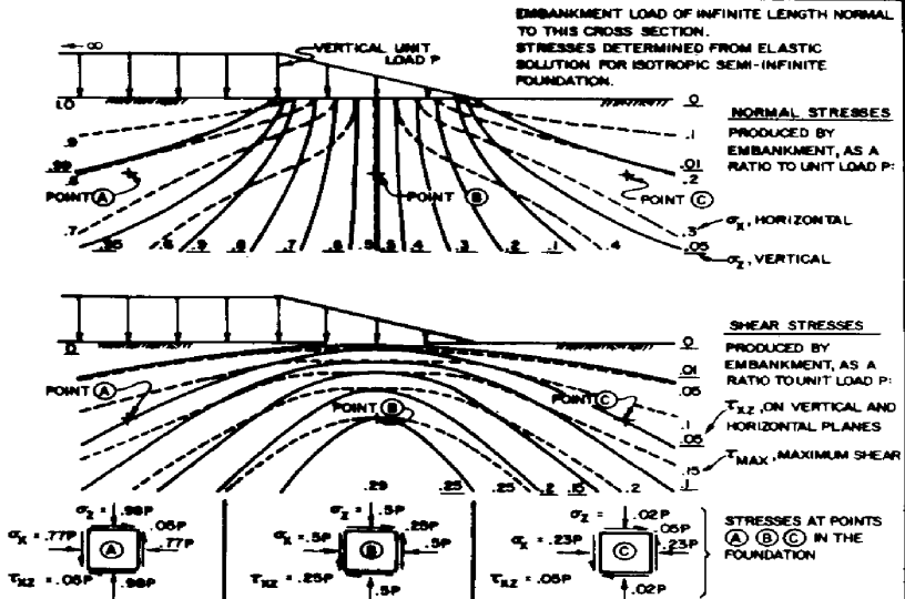
To see all of this “in action” consider the soil stress states shown in Figure 2.

Consider the stress state “A.” The stresses are expressed as a ratio of a pressure P at the surface; furthermore, following geotechnical engineering convention, compressive stresses are positive and the ordinate is the “z” axis.. For this study the convention of Figure 1 will be adopted and thus   .By direct substitution (and carrying the results to precision unjustified in geotechnical engineering) we obtain the following:

• (Equations 12 and 20.)
• (Equations 12 and 20.) Note that the principal stresses are reversed; this is because the sign convention is reversed, and thus what was formerly the smaller of the stresses is now the larger. Also, the axis of the first principal stress changes because the first principal stress itself has changed.
• $latex S=\left[\begin{array}{cc}
  .9754128670 & -.220385433\\
  .2203854365 & .9754128502
  \end{array}\right] $ (Equation 19.) Note that the normalized values of the eigenvectors (Equations 16 and 17) are used. Also note the similarity between this matrix and the Givens rotation matrix of Equation 5.  The diagonalization process is simply a rotation process, as the physics of the problem suggest. (The diagonal terms should be equal to each other and the absolute values ofthe off-diagonal terms should be also; they are not because of numerical errors in Maple where they were computed.
• (Equations 2, 3 and 6.)
• In both cases the trace of A and \Lambda is the same, namely (Equation 21.)

The results are thus the same. The precision is obviously greater than the “slide rule era” Navy [5], but the results illustrate that numerical errors can creep in, even with digital computation.

3. Three-Dimensional Analysis

3.1. Regular Principal Stresses

It is easy to see that, although the concepts are relatively simple, the algebra is involved.It is for this reason that the two-dimensional state was illustrated. With three dimensional stresses, the principles are the same, but the algebra is even more difficult.To begin, one more direction cosine must be defined,

(22)

where is of course the angle of the direction of the rotated coordinate system relative to the original one. The rotated system does not have to be the principal axis system, although that one is of most interest.
For three dimensions, Equation 4 should be written as follows:

$latex \left[\begin{array}{ccc}
\sigma_{x} & \tau_{xy} & \tau_{xz}\\
\tau_{xy} & \sigma_{y} & \tau_{yz}\\
\tau_{xz} & \tau_{yz} & \sigma_{z}
\end{array}\right]\left[\begin{array}{c}
l\\
m\\
n
\end{array}\right]=\left[\begin{array}{c}
p_{x}\\
p_{y}\\
p_{z}
\end{array}\right] $ (23)

All of the moment summations of the shear stresses-which result in the symmetry of the matrix-have been included. The eigenvalues of the matrix are thus the solution of

$latex \left[\begin{array}{ccc}
\sigma_{x}-\lambda & \tau_{xy} & \tau_{xz}\\
\tau_{xy} & \sigma_{y}-\lambda & \tau_{yz}\\
\tau_{xz} & \tau_{yz} & \sigma_{z}-\lambda
\end{array}\right]=0 $ (24)

The characteristic equation of this matrix-and thus the equation that solves for the eigenvalues-is

(25)

where

(26)

(27)

(28)

It is easy to show the following:

• Equation 26 reduces to Equation 9 if .
• Equation 27 reduces to Equation 10 if additionally .
• For all three conditions, Equation 25 reduces to 11.

From the previous derivation, we can thus expect

(29)
(30)
(31)
Solving a cubic equation such as this can be accomplished using the Cardan Formula. Generally, it is possible that we will end up with complex roots, but because of the properties of the matrix we are promised real roots. The eigenvalues are as follows:

$latex \lambda_{1}  =  1/6\,\sqrt[3]{36\,J_{{2}}J_{{1}}-108\,J_{{3}}-8\,{J_{{1}}}^{3}+12\,\sqrt{12\,{J_{{2}}}^{3}-3\,{J_{{2}}}^{2}{J_{{1}}}^{2}-54\,J_{{2}}J_{{1}}J_{{3}}+81\,{J_{{3}}}^{2}+12\,J_{{3}}{J_{{1}}}^{3}}}\nonumber \\
-6\,{\frac{1/3\,J_{{2}}-1/9\,{J_{{1}}}^{2}}{\sqrt[3]{36\,J_{{2}}J_{{1}}-108\,J_{{3}}-8\,{J_{{1}}}^{3}+12\,\sqrt{12\,{J_{{2}}}^{3}-3\,{J_{{2}}}^{2}{J_{{1}}}^{2}-54\,J_{{2}}J_{{1}}J_{{3}}+81\,{J_{{3}}}^{2}+12\,J_{{3}}{J_{{1}}}^{3}}}}}-1/3\,J_{{1}} $ (32)

$latex \lambda_{2}  =  -1/12\,\sqrt[3]{36\,J_{{2}}J_{{1}}-108\,J_{{3}}-8\,{J_{{1}}}^{3}+12\,\sqrt{12\,{J_{{2}}}^{3}-3\,{J_{{2}}}^{2}{J_{{1}}}^{2}-54\,J_{{2}}J_{{1}}J_{{3}}+81\,{J_{{3}}}^{2}+12\,J_{{3}}{J_{{1}}}^{3}}}\nonumber \\
+3\,{\frac{1/3\,J_{{2}}-1/9\,{J_{{1}}}^{2}}{\sqrt[3]{36\,J_{{2}}J_{{1}}-108\,J_{{3}}-8\,{J_{{1}}}^{3}+12\,\sqrt{12\,{J_{{2}}}^{3}-3\,{J_{{2}}}^{2}{J_{{1}}}^{2}-54\,J_{{2}}J_{{1}}J_{{3}}+81\,{J_{{3}}}^{2}+12\,J_{{3}}{J_{{1}}}^{3}}}}}\nonumber \\
-1/3\,J_{{1}}+1/12\,\sqrt{-3}\sqrt[3]{36\,J_{{2}}J_{{1}}-108\,J_{{3}}-8\,{J_{{1}}}^{3}+12\,\sqrt{12\,{J_{{2}}}^{3}-3\,{J_{{2}}}^{2}{J_{{1}}}^{2}-54\,J_{{2}}J_{{1}}J_{{3}}+81\,{J_{{3}}}^{2}+12\,J_{{3}}{J_{{1}}}^{3}}}\nonumber \\
+2\sqrt{-3}\,{\frac{1/3\,J_{{2}}-1/9\,{J_{{1}}}^{2}}{\sqrt[3]{36\,J_{{2}}J_{{1}}-108\,J_{{3}}-8\,{J_{{1}}}^{3}+12\,\sqrt{12\,{J_{{2}}}^{3}-3\,{J_{{2}}}^{2}{J_{{1}}}^{2}-54\,J_{{2}}J_{{1}}J_{{3}}+81\,{J_{{3}}}^{2}+12\,J_{{3}}{J_{{1}}}^{3}}}}} $ (33)

$latex \lambda_{3} =  -1/12\,\sqrt[3]{36\,J_{{2}}J_{{1}}-108\,J_{{3}}-8\,{J_{{1}}}^{3}+12\,\sqrt{12\,{J_{{2}}}^{3}-3\,{J_{{2}}}^{2}{J_{{1}}}^{2}-54\,J_{{2}}J_{{1}}J_{{3}}+81\,{J_{{3}}}^{2}+12\,J_{{3}}{J_{{1}}}^{3}}}\nonumber \\
+3\,{\frac{1/3\,J_{{2}}-1/9\,{J_{{1}}}^{2}}{\sqrt[3]{36\,J_{{2}}J_{{1}}-108\,J_{{3}}-8\,{J_{{1}}}^{3}+12\,\sqrt{12\,{J_{{2}}}^{3}-3\,{J_{{2}}}^{2}{J_{{1}}}^{2}-54\,J_{{2}}J_{{1}}J_{{3}}+81\,{J_{{3}}}^{2}+12\,J_{{3}}{J_{{1}}}^{3}}}}}\nonumber \\
-1/3\,J_{{1}}-1/12\,\sqrt{-3}\sqrt[3]{36\,J_{{2}}J_{{1}}-108\,J_{{3}}-8\,{J_{{1}}}^{3}+12\,\sqrt{12\,{J_{{2}}}^{3}-3\,{J_{{2}}}^{2}{J_{{1}}}^{2}-54\,J_{{2}}J_{{1}}J_{{3}}+81\,{J_{{3}}}^{2}+12\,J_{{3}}{J_{{1}}}^{3}}}\nonumber \\
-2\sqrt{-3}\,{\frac{1/3\,J_{{2}}-1/9\,{J_{{1}}}^{2}}{\sqrt[3]{36\,J_{{2}}J_{{1}}-108\,J_{{3}}-8\,{J_{{1}}}^{3}+12\,\sqrt{12\,{J_{{2}}}^{3}-3\,{J_{{2}}}^{2}{J_{{1}}}^{2}-54\,J_{{2}}J_{{1}}J_{{3}}+81\,{J_{{3}}}^{2}+12\,J_{{3}}{J_{{1}}}^{3}}}}} $ (34)

3.2. Deviatoric Principal Stresses

The algebra of Equations 32, 33 and 34 is rather involved. Is there a way to simplify it? The answer is”yes” if we use a common reduction of the Cardan Formula. Consider the following change of variables:

(35)

(36)

(37)

Since the change is the same in all directions, we can write

$latex \left[\begin{array}{ccc}
\sigma’_{x} & \tau_{xy} & \tau_{xz}\\
\tau_{xy} & \sigma’_{y} & \tau_{yz}\\
\tau_{xz} & \tau_{yz} & \sigma’_{z}
\end{array}\right]\left[\begin{array}{c}
l\\
m\\
n
\end{array}\right]=\left[\begin{array}{c}
p’_{x}\\
p’_{y}\\
p’_{z}
\end{array}\right] $ (38)

and

$latex \left[\begin{array}{ccc}
\sigma’_{x}-\lambda’ & \tau_{xy} & \tau_{xz}\\
\tau_{xy} & \sigma’_{y}-\lambda’ & \tau_{yz}\\
\tau_{xz} & \tau_{yz} & \sigma’_{z}-\lambda’
\end{array}\right]=0 $ (39)

The characteristic equation of the matrix in Equation 39 is

(40)
where

(41)

(42)

Although our motivation for this was to simplify the characteristic equation, the deviatoric stress infact has physical significance. As Jaeger and Cook [4] point out, “…essentially ( ) determines uniform compression or dilation, while the stress deviation determines distortion. Since many criteria of failure are concerned primarily with distortion, and since they must be invariant with respect to rotation of axes, it appears that the invariants of stress deviation will be involved.”

The one thing to be careful about is that the eigenvalues from Equation 24 are not the same as those from Equation 39. The latter are in fact “deviatoric eigenvalues” and are equivalent to deviatoric principal stresses, thus

(43)

(44)

(45)

These can be converted back to full stresses using Equations 35, 36 and 37. The eigenvalues for the deviatoric stresses are

  (46)

$latex \lambda’_{2} = -1/12\,\sqrt[3]{108\,J’_{{3}}+12\,\sqrt{-12\,{J’_{{2}}}^{3}+81\,{J’_{{3}}}^{2}}}-{\frac{J’_{{2}}}{\sqrt[3]{108\,J’_{{3}}+12\,\sqrt{-12\,{J’_{{2}}}^{3}+81\,{J’_{{3}}}^{2}}}}}\nonumber \\
+1/2\,\sqrt{-1}\sqrt{3}\left(1/6\,\sqrt[3]{108\,J’_{{3}}+12\,\sqrt{-12\,{J’_{{2}}}^{3}+81\,{J’_{{3}}}^{2}}}-2\,{\frac{J’_{{2}}}{\sqrt[3]{108\,J’_{{3}}+12\,\sqrt{-12\,{J’_{{2}}}^{3}+81\,{J’_{{3}}}^{2}}}}}\right) $ (47)

$latex \lambda’_{3} = -1/12\,\sqrt[3]{108\,J’_{{3}}+12\,\sqrt{-12\,{J’_{{2}}}^{3}+81\,{J’_{{3}}}^{2}}}-{\frac{J’_{{2}}}{\sqrt[3]{108\,J’_{{3}}+12\,\sqrt{-12\,{J’_{{2}}}^{3}+81\,{J’_{{3}}}^{2}}}}}\nonumber \\
-1/2\,\sqrt{-1}\sqrt{3}\left(1/6\,\sqrt[3]{108\,J’_{{3}}+12\,\sqrt{-12\,{J’_{{2}}}^{3}+81\,{J’_{{3}}}^{2}}}-2\,{\frac{J’_{{2}}}{\sqrt[3]{108\,J’_{{3}}+12\,\sqrt{-12\,{J’_{{2}}}^{3}+81\,{J’_{{3}}}^{2}}}}}\right) $ (48)

Solving Equations 24 and 39 will yield eigenvalues and principal stresses of one kind or another. The eigenvectors and direction cosines can be determined using the same methods used for the two-dimensional problem. It should be readily evident, however, that the explicit solution of these eivenvectors and diagonalizing rotational matrices is very involved, although using deviatoric stresses simplifies the algebra considerably. If the material is isotropic, and its properties are the same in all directions, than the direction of the principal stresses can frequently be neglected. For anisotropic materials, this is not the case.

4. Finding the Eigenvalues and Eigenvectors Using the Method of Danilevsky

For the simple 3 * 3 matrix, computing the determinant, and from it the the invariants, is not a major task. With larger matrices, it is far more difficult to find the determinant, let alone the characteristic polynomial.There have been many solutions to this problem over the years. For larger matrices the most common are Householder reflections and/or Givens rotations. We discussed the latter earlier. By doing multiple reflections and/or rotations, the matrix can be diagonalized and the eigenvalues “magically appear.” The whole problem of solving the characteristic equation is avoided, although the iterative cost in getting to the result can be considerable.

The method we’ll explore here is that of Danilevsky, first published in 1937, as presented in Faddeeva [3].

4.1. Theory

The math will be presented in format, but it can be expanded to any size square matrix. The idea is, through a series of similarity transformations, to transform a matrix (such as is shown in Equation 23) to the Frobenius normal form, which is

$latex D=\left[\begin{array}{ccc}
p_{{1}} & p_{{2}} & p_{{3}}\\
\noalign{\medskip}1 & 0 & 0\\
\noalign{\medskip}0 & 1 & 0
\end{array}\right] $ (49)

From here we take the determinant of , thus

$latex D\left(\lambda\right)=\left|\begin{array}{ccc}
p_{1}-\lambda & p_{2} & p_{3}\\
1 & -\lambda & 0\\
0 & 1 & -\lambda
\end{array}\right| $ (50)

The determinant-and thus the characteristic polynomial-is easy to compute, and setting it equal to zero,

(51)

This is obviously the same as Equation 25, but now we can read the invariants straight out of the similar matrix.

So how do we get to Equation 49? The simple answer is through a series of row reductions. We start for the matrix by carrying the third row into the second, dividing all the elements by the element in the last row by the element , then subtracting the second column, multiplied by respectively from all the rest of the columns. Row and column manipulation is common with computational matrix routines, but a more straightforward way is to postmultiply by the matrix

$latex M=\left[\begin{array}{ccc}
1 & 0 & 0\\
\noalign{\medskip}-{\frac{a_{{3,1}}}{a_{{3,2}}}} & {a_{{3,2}}}^{-1} & -{\frac{a_{{3,3}}}{a_{{3,2}}}}\\
\noalign{\medskip}0 & 0 & 1
\end{array}\right] $ (52)

The result will not be similar to , but if we premultiply that result by ,

$latex M^{-1}=\left[\begin{array}{ccc}
1 & 0 & 0\\
\noalign{\medskip}a_{{3,1}} & a_{{3,2}} & a_{{3,3}}\\
\noalign{\medskip}0 & 0 & 1
\end{array}\right] $ (53)

that result will be by Equation 19, although does not diagonalize the result the way did. Performing this series of matrix multplications yields

$latex B=M^{-1}AM=\left[\begin{array}{ccc}
a_{{1,1}}-{\frac{a_{{1,2}}a_{{3,1}}}{a_{{3,2}}}} & {\frac{a_{{1,2}}}{a_{{3,2}}}} & -{\frac{a_{{1,2}}a_{{3,3}}}{a_{{3,2}}}}+a_{{1,3}}\\
\noalign{\medskip}a_{{3,1}}\left(a_{{1,1}}-{\frac{a_{{1,2}}a_{{3,1}}}{a_{{3,2}}}}\right)+a_{{3,2}}\left(a_{{2,1}}-{\frac{a_{{2,2}}a_{{3,1}}}{a_{{3,2}}}}\right) & {\frac{a_{{1,2}}a_{{3,1}}}{a_{{3,2}}}}+a_{{2,2}}+a_{{3,3}} & a_{{3,1}}\left(-{\frac{a_{{1,2}}a_{{3,3}}}{a_{{3,2}}}}+a_{{1,3}}\right)+a_{{3,2}}\left(-{\frac{a_{{2,2}}a_{{3,3}}}{a_{{3,2}}}}+a_{{2,3}}\right)\\
\noalign{\medskip}0 & 1 & 0
\end{array}\right] $ (54)

We continue this process by moving up a row, thus the new similarity transformation matrices are

$latex N  =  \left[\begin{array}{ccc}
{b_{{2,1}}}^{-1} & -{\frac{b_{{2,2}}}{b_{{2,1}}}} & -{\frac{b_{{2,3}}}{b_{{2,1}}}}\\
\noalign{\medskip}0 & 1 & 0\\
\noalign{\medskip}0 & 0 & 1
\end{array}\right] $ (55)

$latex N^{-1}  =  \left[\begin{array}{ccc}
b_{{2,1}} & b_{{2,2}} & b_{{2,3}}\\
\noalign{\medskip}0 & 1 & 0\\
\noalign{\medskip}0 & 0 & 1
\end{array}\right] $ (56)

Although we formed the M and N matrices first, from a conceptual and computational standpoint itis easier to form the “inverse” matrices first and then invert them. One drawback to Danilevsky’s method is that there are many opportunities for division by zero, which need to be taken into consideration when employing the method.

In any case the next step yields

$latex C=N^{-1}BN=\left[\begin{array}{ccc}
b_{{1,1}}+b_{{2,2}} & b_{{2,1}}\left(-{\frac{b_{{1,1}}b_{{2,2}}}{b_{{2,1}}}}+b_{{1,2}}\right)+b_{{2,3}} & b_{{2,1}}\left(-{\frac{b_{{1,1}}b_{{2,3}}}{b_{{2,1}}}}+b_{{1,3}}\right)\\
\noalign{\medskip}1 & 0 & 0\\
\noalign{\medskip}0 & 1 & 0
\end{array}\right] $ (57)

From this Equation 49 is easily formed.
The coefficients and are simply the invariants, which have already been established earlier for both standard and deviatoric normal stresses. From that standpoint the method seems to be overkill.

The advantage comes when we compute the eigenvectors/direction cosines. Consider the vector

$latex y=\left[\begin{array}{c}
y_{1}\\
y_{2}\\
y_{3}
\end{array}\right] $ (58)

Premultiplying it by (see Equation 50) yields

$latex \left[\begin{array}{ccc}
p_{1}-\lambda & p_{2} & p_{3}\\
1 & -\lambda & 0\\
0 & 1 & -\lambda
\end{array}\right]\left[\begin{array}{c}
y_{1}\\
y_{2}\\
y_{3}
\end{array}\right]=\left[\begin{array}{c}
\left(p_{{1}}-\lambda\right)y_{{1,1}}+p_{{2}}y_{{2,1}}+p_{{3}}y_{{3,1}}\\
\noalign{\medskip}y_{{1,1}}-\lambda\,y_{{2,1}}\\
\noalign{\medskip}y_{{2,1}}-\lambda\,y_{{3,1}}
\end{array}\right]=0 $ (59)

For y to be non-trivial,

$latex y=\left[\begin{array}{c}
\lambda^{2}\\
\lambda\\
1
\end{array}\right] $ (60)

It can be shown (Faddeeva [3]) that the eigenvectors can be found as follows (successive rotations:)

$latex \bar{x}_{n}=MNy=\left[\begin{array}{c}
{\frac{{\lambda_{n}}^{2}}{b_{{2,1}}}}-{\frac{b_{{2,2}}\lambda_{n}}{b_{{2,1}}}}-{\frac{b_{{2,3}}}{b_{{2,1}}}}\\
\noalign{\medskip}-a_{{3,1}}\left({\frac{{\lambda_{n}}^{2}}{b_{{2,1}}}}-{\frac{b_{{2,2}}\lambda_{n}}{b_{{2,1}}}}-{\frac{b_{{2,3}}}{b_{{2,1}}}}\right){a_{{3,2}}}^{-1}+{\frac{\lambda_{n}}{a_{{3,2}}}}-{\frac{a_{{3,3}}}{a_{{3,2}}}}\\
\noalign{\medskip}1
\end{array}\right] $ (61)

These can, as was shown earlier, be normalized to direction cosines and can form the diagonalizing matrices.

4.2. Three-Dimensional Example

An example of this is drawn from Boresi et al. [1]. It involves a stress state, which referring to Equation 23 can be written (all stresses in kPa) as

$latex A=\left[\begin{array}{ccc}
120 & -55 & -75\\
\noalign{\medskip}-55 & 55 & 33\\
\noalign{\medskip}-75 & 33 & -85
\end{array}\right] $ (62)

For the first transformation, we substitute these values into Equation 54 and thus

$latex B=\left[\begin{array}{ccc}
1 & 0 & 0\\
\noalign{\medskip}-75 & 33 & -85\\
\noalign{\medskip}0 & 0 & 1
\end{array}\right]\left[\begin{array}{ccc}
120 & -55 & -75\\
\noalign{\medskip}-55 & 55 & 33\\
\noalign{\medskip}-75 & 33 & -85
\end{array}\right]\left[\begin{array}{ccc}
1 & 0 & 0\\
\noalign{\medskip}{\frac{25}{11}} & 1/33 & {\frac{85}{33}}\\
\noalign{\medskip}0 & 0 & 1
\end{array}\right]=\left[\begin{array}{ccc}
-5 & -5/3 & -{\frac{650}{3}}\\
\noalign{\medskip}2685 & 95 & 22014\\
\noalign{\medskip}0 & 1 & 0

\end{array}\right] $ (63)

The second transformation, following Equation 57,

$latex C=\left[\begin{array}{ccc}
2685 & 95 & 22014\\
\noalign{\medskip}0 & 1 & 0\\
\noalign{\medskip}0 & 0 & 1
\end{array}\right]\left[\begin{array}{ccc}
-5 & -5/3 & -{\frac{650}{3}}\\
\noalign{\medskip}2685 & 95 & 22014\\
\noalign{\medskip}0 & 1 & 0
\end{array}\right]\left[\begin{array}{ccc}
{\frac{1}{2685}} & -{\frac{19}{537}} & -{\frac{7338}{895}}\\
\noalign{\medskip}0 & 1 & 0\\
\noalign{\medskip}0 & 0 & 1
\end{array}\right]=\left[\begin{array}{ccc}
90 & 18014 & -471680\\
\noalign{\medskip}1 & 0 & 0\\
\noalign{\medskip}0 & 1 & 0
\end{array}\right] $ (64)

From this the characteristic equation is, from Equation 51,

(65)

which yields eigenvalues/principal stresses of 176.8, 24.06 and -110.86 kPa.

So how does this look with deviatoric stresses? Applying Equations 26, 35, 36 and 37 yields

$latex A’=\left[\begin{array}{ccc}
90 & -55 & -75\\
\noalign{\medskip}-55 & 25 & 33\\
\noalign{\medskip}-75 & 33 & -115
\end{array}\right] $ (66)

It’s worth noting that, for the deviatoric stress matrix, the trace is always zero. The two similarity transformations are thus:

$latex B’  =  \left[\begin{array}{ccc}
1 & 0 & 0\\
\noalign{\medskip}-75 & 33 & -115\\
\noalign{\medskip}0 & 0 & 1
\end{array}\right]\left[\begin{array}{ccc}
90 & -55 & -75\\
\noalign{\medskip}-55 & 25 & 33\\
\noalign{\medskip}-75 & 33 & -115
\end{array}\right]\left[\begin{array}{ccc}
1 & 0 & 0\\
\noalign{\medskip}{\frac{25}{11}} & 1/33 & {\frac{115}{33}}\\
\noalign{\medskip}0 & 0 & 1
\end{array}\right]=\left[\begin{array}{ccc}
-35 & -5/3 & -{\frac{800}{3}}\\
\noalign{\medskip}2685 & 35 & 23964\\
\noalign{\medskip}0 & 1 & 0
\end{array}\right] $ (67)

$latex C’ =  \left[\begin{array}{ccc}
2685 & 35 & 23964\\
\noalign{\medskip}0 & 1 & 0\\
\noalign{\medskip}0 & 0 & 1
\end{array}\right]\left[\begin{array}{ccc}
-35 & -5/3 & -{\frac{800}{3}}\\
\noalign{\medskip}2685 & 35 & 23964\\
\noalign{\medskip}0 & 1 & 0
\end{array}\right]\left[\begin{array}{ccc}
{\frac{1}{2685}} & -{\frac{7}{537}} & -{\frac{7988}{895}}\\
\noalign{\medskip}0 & 1 & 0\\
\noalign{\medskip}0 & 0 & 1
\end{array}\right]=\left[\begin{array}{ccc}
0 & 20714 & 122740\\
\noalign{\medskip}1 & 0 & 0\\
\noalign{\medskip}0 & 1 & 0
\end{array}\right] $ (68)

and the characteristic polynomial (missing the squared term, as expected)

(69)

which yields eigenvalues/principal deviatoric stresses of 146.8, -5.94 and -140.86 kPa.

4.3. Numerical Implementation

Even with a “simple” problem such as this, the algebra of the solution can become very involved. Moreover, as is frequently the case with numerical linear algebra, there are two “loose ends” that need to be tied up: the division by zero problem in Danilevsky’s Method, and solving for the eigenvalues/principal stresses. A numerical implementation, shown below, will address both issues, if not completely.

The FORTRAN 77 code is in the appendix. It is capable of solving the problem both for standard and deviatoric stresses. The example problem given above is used. The steps used are as follows:

1. If deviatoric stresses are specified, the normal stresses are accordingly converted as shown earlier.
2. The invariants are computed. For a more general routine of Danilevsky’s Method, the matrices associated with the similarity transformations-and their inverses-would have to be computed and the matrix multiplications done. In this case the results of these multiplications-the invariants themselves-are “hard coded” into the routine, which saves a great deal of matrix multiplication. It also eliminated problems with division by zero up to this point.
3. The eigenvalues/principal stresses are computed using Newton’s Method. Obviously they could be computed analytically as shown earlier. For this type of problem, this is possible; for characteristic polynomials beyond degree four, another type of solution is necessary. The major problem with New-ton’s Method is picking initial values so as to yield distinct eigenvalues. The nature of the problem suggests that the initial normal, diagonal stresses can be used as starting values. For the sample problem this worked out very well; it was not tested on a variety of stress states.
4. Taking the three resulting eigenvalues, the eigenvectors were computed using Equation 61. Again the matrix multiplications were hard-coded into the routine. The problem of division by zero of certain values of shear stresses was not addressed. In some cases Equation 61 will result in division by zero.The eigenvectors were then normalized, which yielded three sets of direction cosines.

The results for the regular stresses are shown in Figure 3 and those for deviatoric stresses are shown in Figure 4.

The principal stress results agree with the “hand” calculations earlier. The direction cosines-and thus the diagonalizing matrices-are the same for both cases.

5. Conclusion

We have explored the analysis of Mohr’s Circle for stress states in both two and three dimensions.The equations can be derived from strictly linear algebra considerations, the principal stresses being the eigenvalues and the direction cosines being the normalized eigenvectors. It was also shown that numericalmethods can be employed to analyze these results and the invariants, in this case using the computationally efficient Danilevsky’s Method.

Note: since we first published this on a companion site two years ago, we have made several improvements to the methods described here.  These can be found in this post.

Appendix: Source Code for Numerical Implementation

! Routine to Determine Stress State from Danilevsky's Method
! Taken from Faddeeva (1959) with Example Case from Boresi et.al. (1993)
! Define Variables for Test Case
CHARACTER*12 filnam
sigmax=120.
sigmay=55.
sigmaz=-85.
tauxy=-55.
tauyz=33.
tauxz=-75.
! Set Variable for Eigenvalue Solution
! ityp = 0 Regular
! ityp = 1 Deviatoric
WRITE (6,*) 'Standard (0) or Deviatoric (1) Stress:'
READ (5,*) ityp
IF (ityp.eq.0) filnam='danil0.txt'
IF (ityp.eq.1) filnam='danil1.txt'
! Open Output File
OPEN (7,file=filnam)
CALL danil (sigmax, sigmay, sigmaz, tauxy, tauyz, tauxz, ityp)
CLOSE (7)
STOP
END

! Subroutine danil -- Danilevsky's Method specifically written
! for 3 x 3 matrices and stress-state solution
SUBROUTINE danil (sigmax, sigmay, sigmaz, tauxy, tauyz, tauxz,
&ityp)
REAL p(3),x(3,3),sigma(3),i1,lambda
! Convert Normal Stresses to Deviatoric Stresses if ityp = 1
IF (ityp.eq.1) THEN
i1=0.3333333333*(sigmax+sigmay+sigmaz)
sigmax=sigmax-i1
sigmay=sigmay-i1
sigmaz=sigmaz-i1
END IF
! Compute Invariants
IF (ityp.eq.0) p(1)=sigmax+sigmay+sigmaz
IF (ityp.eq.1) p(1)=0.0
p(2)=-sigmax*sigmay-sigmax*sigmaz+tauxy**2+tauxz**2-sigmay*sigmaz+
&tauyz**2
p(3)=sigmax*sigmay*sigmaz-sigmax*tauyz**2+2*tauxy*tauxz*tauyz-
&tauxy**2*sigmaz-tauxz**2*sigmay
! Use Newton's Method to Determine Eigenvalues
DO 60 j=1,3,1
GO TO (10,20,30),j
10 lambda=sigmax
GO TO 40
20 lambda=sigmay
GO TO 40
30 lambda=sigmaz
40 DO 50 i=1,10,1
fun=lambda**2*p(1)-lambda**3+p(2)*lambda+p(3)
der=2*lambda*p(1)-3*lambda**2+p(2)
lambda=lambda-fun/der
delta=abs(fun/lambda)
IF (delta.lt.1.0e-5) GO TO 60
50 CONTINUE
60 sigma(j)=lambda
! Determine Eigenvectors
DO 80 i=1,3,1
lambda=sigma(i)
x(1,i)=-1/(-tauxz*sigmax*tauyz+tauxy*tauxz**2-tauxy*tauyz**2+
& tauyz*sigmay*tauxz)*tauyz*lambda**2+(tauxy*tauxz+sigmay*tauyz+
& sigmaz*tauyz)/(-tauxz*sigmax*tauyz+tauxy*tauxz**2-tauxy*tauyz**
& 2+tauyz*sigmay*tauxz)*lambda-(tauxz*tauxy*sigmaz-tauyz*tauxz**
& 2+tauyz*sigmay*sigmaz-tauyz**3)/(-tauxz*sigmax*tauyz+tauxy*
& tauxz**2-tauxy*tauyz**2+tauyz*sigmay*tauxz)
x(2,i)=-tauxz/tauyz*(-1/(-tauxz*sigmax*tauyz+tauxy*tauxz**2-
& tauxy*tauyz**2+tauyz*sigmay*tauxz)*tauyz*lambda**2+(tauxy*
& tauxz+sigmay*tauyz+sigmaz*tauyz)/(-tauxz*sigmax*tauyz+tauxy*
& tauxz**2-tauxy*tauyz**2+tauyz*sigmay*tauxz)*lambda-(tauxz*
& tauxy*sigmaz-tauyz*tauxz**2+tauyz*sigmay*sigmaz-tauyz**3)/(-
& tauxz*sigmax*tauyz+tauxy*tauxz**2-tauxy*tauyz**2+tauyz*sigmay*
& tauxz))+1/tauyz*lambda-sigmaz/tauyz
x(3,i)=1.0
! Normalise Eigenvectors
xnorm=1.0/sqrt(x(1,i)**2+x(2,i)**2+x(3,i)**2)
DO 70 j=1,3,1
70 x(j,i)=x(j,i)*xnorm
80 CONTINUE
! Write Results
WRITE (7,*) 'Stress State Using Danilevskys Method:'
IF (ityp.eq.0) WRITE (7,*) 'Regular Normal Stresses'
IF (ityp.eq.1) WRITE (7,*) 'Deviatoric Normal Stresses'
WRITE (7,*) 'Original Stress Matrix/Tensor:'
WRITE (7,100) sigmax,tauxy,tauxz
WRITE (7,100) tauxy,sigmay,tauyz
WRITE (7,100) tauxz,tauyz,sigmaz
WRITE (7,*) 'Invariants:'
WRITE (7,100) (p(j),j=1,3,1)
WRITE (7,*) 'Principal Stresses:'
WRITE (7,100) (sigma(j),j=1,3,1)
WRITE (7,*) 'Direction Cosines:'
DO 90 j=1,3,1
90 WRITE (7,110) (x(j,i),i=1,3,1)
100 FORMAT (3f15.2)
110 FORMAT (3f15.3)
RETURN
END

References

[1] Boresi, A. P., Schmidt, R. J., Sidebottom, O. M., 1993. Advanced Mechanics of Materials, 5th Edition.John Wiley & Sons, Inc.

[2] DeRusso, P., Roy, R., Close, C., 1965. State Variables for Engineers. John Wiley & Sons, Inc., New York,NY.

[3] Faddeeva, V., 1959. Computational Methods of Linear Algebra. Dover Publications, Inc.

[4] Jaeger, J., Cook, N., 1979. Fundamentals of Rock Mechanics, 3rd Edition. Chapman and Hall.

[5] Navy, U., 1986. Soil mechanics. Tech. Rep. DM 7.01.

[6] Owen, D., Hinton, E., 1980. Finite Elements in Plasticity: Theory and Practice. Pineridge Press, Swansea,Wales.

[7] Strang, G., 1993. Introduction to Linear Algebra. Wellesley-Cambridge Press.

[8] Verruijt, A., van Bars, S., 2007. Soil Mechanics. VSSD, The Netherlands.