
The object of this is to solve the differential equation

for the following boundary conditions and parameters:


Conventional wisdom would indicate that, because of the high order of the derivatives, this problem cannot be solved using a scalar implementation of simple shooting. However, this is not the case.
To see why this is so, let us begin by implementing the following notation:


If we substitute these into the differential equation and solve for the third derivative, we have

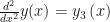
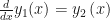
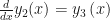
Now we can construct a series of first-order differential equations for our Runge-Kutta integration scheme as follows:

Now let us consider things at our first boundary point, namely

Making the appropriate substitutions yields

We thus see that, if we use 


which goes to zero as the far boundary condition is met.
To implement this we used a same simple shooting routine with a regula falsi root-finding technique. One thing that was varied was the number of integration steps in the interval; we wanted to see how this affected the convergence.
The results of this are summarized below.
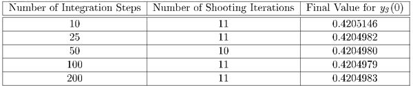 The number of shooting iterations is fairly constant with the variation in integration steps; however, the final value of
A plot of the results is shown below.
 FORTRAN 77 code is below. Some of the “includes”, subroutines and functions are as follows:
- matsize.for is a brief snippet of code which includes a parameter statement which sizes the variable size arrays.
- tstamp calls an OPEN WATCOM routine that returns the date and time and places it in the output.
- scrsho is a “line plotter” routine, very old school.
c Solution of Third-Order Ordinary Differential Equation
 c Using Simple Shooting Method and Regula Falsi root-finding technique
 c Solution based on Carnahan, Luther and Wilkes (1969)
 include 'matsize.for'
 parameter(neqs=3,nx=10)
 character*40 vinput(nmax)
 character*16 voutpt(nmax)
 c Plot title
 character*60 titlep
 dimension y(neqs),dy(neqs),xyplot(0:nx,2)
 c Define third derivative function
 y4(y1,y2,y3,xmu)=xmu*y3-xmu*y3*y1**2-2.*xmu*y1*y2**2-y2
 c Define second boundary condition function
 bfin(y1,y1fin)=y1-y1fin
 c Enter Boundary Conditions
 data y1strt/0.0/,y2strt/0.5/,y1fin/1.0/xstrt/0.0/,xend/2.0/
 c Enter initial upper and lower bounds for y(3) (Second Derivative)
 data y3left/2.0/,y3rite/0.0/
 c Enter number of shots
 data n/50/
 c Enter friction coefficient
 data xmu/0.5/
 c Enter nomenclature describing initial data as data statements
 data vinput(1)/'Left Initial Bracket'/
 data vinput(2)/'Right Initial Bracket'/
 data vinput(4)/'Delta x increment'/
 data vinput(5)/'First Boundary Condition'/
 data vinput(6)/'Second Boundary Condition'/
 data vinput(7)/'mu'/
 data vinput(8)/'Number of Shots'/
 c Enter nomenclature describing output for individual case
 data vinput(11)/'Shot Number'/
 data vinput(12)/'Value of Guess for Second Derivative'/
 data voutpt(1)/'x'/
 data voutpt(2)/'y(x)'/
 data voutpt(3)/'y`(x)'/
 data voutpt(4)/'y``(x)'/
 data voutpt(5)/'y```(x)'/
 data titlep/'Plot of Final Boundary Condition vs. x'/
 c Description of variables below the comment:
 write(*,*)'Math 5610 Spring 2012 Final Exam'
 write(*,*)'Simple Shooting Method for Third-Order ODE'
 call tstamp
 c Compute value of integration step size for dx
 dx = (xend-xstrt)/float(nx)
 write(*,*)
 c Interval of uncertainty (left)
 1 write(*,*)'Initial Parameters for Problem:'
 write(*,200)vinput(1),y3left
 c Interval of uncertainty (right)
 write(*,200)vinput(2),y3rite
 write(*,200)vinput(4),dx
 write(*,200)vinput(5),xstrt
 write(*,200)vinput(6),xend
 write(*,200)vinput(7),xmu
 write(*,200)vinput(8),n
 do 21 iter=1,n,1
 c ..... Set and print initial conditions
 c ..... Since regula falsi isn't "self starting" it is necessary
 c to compute the left and right values for y(3) (regula
 c falsi independent variable) and compute the corresponding
 c result for bfnact (regula falsi dependent variable)
 c
 c This is done in the first two iterations
 c Iteration 1: Right Value
 c Iteration 2: Left Value
 c Susequent iterations adjust boundaries according to the
 c method
 x = xstrt
 y(1)=y1strt
 y(2)=y2strt
 if(iter.eq.1)then
 y(3) = y3rite
 write(*,*)'Iteration for Right Estimate'
 elseif(iter.eq.2)then
 y(3) = y3left
 write(*,*)'Iteration for Left Estimate'
 else
 y(3) = (y3left*bfinr-y3rite*bfinl)/(bfinr-bfinl)
 endif
 bfnold =bfnact
 y3zero = y(3)
 c Set print index to zero; print index changed at the first, middle
 c and last iteration and printing/plotting takes place
 write(*,*)
 write(*,210)iter
 write(*,200)vinput(1),y3left
 write(*,200)vinput(12),y3zero
 write(*,200)vinput(2),y3rite
 write(*,*)
 write(*,212)(voutpt(np),np=1,5,1)
 write(*,*)
 bfnact=bfin(y(1),y1fin)
 write(*,202)x,y(1),y(2),y(3),bfnact
 c ..... Set Selected variable for plot routine
 xyplot(0,1)=x
 xyplot(0,2)=bfnact
 do 17 icycle=1,nx,1
 c ..... Call Runge-Kutta Subroutine .....
 8 if(irunge(neqs,y,dy,x,dx).ne.1)goto 10
 dy(1)=y(2)
 dy(2)=y(3)
 dy(3)=y4(y(1),y(2),y(3),xmu)
 goto 8
 c ..... Print Solutions, Plot bfnact vs. x values .....
 10 bfnact=bfin(y(1),y1fin)
 write(*,202)x,y(1),y(2),y(3),bfnact
 c ..... Set Selected variable for plot routine
 nplot = icycle
 xyplot(icycle,1)=x
 xyplot(icycle,2)=bfnact
 if(icycle.eq.nx)call scrsho(xyplot,nx,titlep)
 17 continue
 c ..... Ending routine if difference between current and past
 c values of the boundary condition function are small enough
 if(iter.eq.1)then
 bfinr=bfnact
 elseif(iter.eq.2)then
 bfinl=bfnact
 else
 err = abs((bfnold-bfnact)/xmu)
 if(err.lt.1.0e-06)goto 23
 if(bfnact*bfinl.gt.0)then
 y3left = y3zero
 bfinl = bfnact
 else
 y3rite = y3zero
 bfinr = bfnact
 endif
 endif
 21 continue
 23 continue
 200 format(A40,2h ,g15.7)
 202 format(1x,f7.4,2f16.7,2f16.8)
 210 format(35hResults for Regula Falsi Iteration ,i2)
 212 format(1x,5a16)
 stop
 end
function irunge(n,y,f,x,h)
 c Fourth-order Runge-Kutta integration routine
 c Taken from Carnahan, Luther and Wilkes (1969)
 c
 c The function irunge employs the fourth-order Runge-Kutta method
 c with Kutta's coefficients to integrate a system of n simultaneous
 c first-order ordinary differential equations f(j)=dy(j)/dx,
 c (j=1,2,...,n), across one step of length h in the independent
 c variable x, subject to initial conditions y(j), (j=1,2,...,n).
 c Each f(j), the derivative of y(j), must be computed four times
 c per integration step by the calling program. The function must
 c be called five times per step (pass(1)...pass(5)) so that the
 c independent variable value (x) and the solution values (y(1)...y(n))
 c can be updated using the Runge-Kutta algorithm. M is the pass
 c counter. Irunge returns as its value 1 to signal that all derivatives
 c (the f(j)) be evaluated or 0 to signal that the integration process
 c for the current step is finished. Savey(j) is used to save the
 c initial value of y(j) and phi(j) is the increment function for the
 c j(th) equation.
 c
 c The size of the savey and phi arrays depends upon the value of the parameter
 c which is included.
 include 'matsize.for'
 dimension phi(nmax),savey(nmax),y(n),f(n)
 data m/0/
 m=m+1
 goto(1,2,3,4,5), m
 c ..... Pass 1 .....
 1 irunge=1
 return
 c ..... Pass 2 .....
 2 do 22 j=1,n,1
 savey(j)=y(j)
 phi(j)=f(j)
 22 y(j)=savey(j)+h*f(j)/2.0
 x=x+h/2.0
 irunge=1
 return
 c ..... Pass 3 .....
 3 do 33 j=1,n,1
 phi(j)=phi(j)+2.0*f(j)
 33 y(j) = savey(j)+0.5*h*f(j)
 irunge=1
 return
 c ..... Pass 4 .....
 4 do 44 j=1,n,1
 phi(j)=phi(j)+2.0*f(j)
 44 y(j)=savey(j)+h*f(j)
 x=x+0.5*h
 irunge=1
 return
 c ..... Pass 5 .....
 5 do 55 j=1,n,1
 55 y(j)=savey(j)+(phi(j)+f(j))*h/6.0
 m=0
 irunge=0
 return
 end
