Numerical Integration of a Function in a Two-Dimensional Space, and Its Solution with Conjugate Gradient

The purpose of this piece is to document the numerical integration of a function in a two-dimensional space using the conjugate gradient method.

Basic Problem Statement and Closed Form Solution

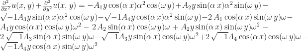
The boundary value problem is as follows:
${\frac{\partial^{2}}{\partial{x}^{2}}}u(x,y)+{\frac{\partial^{2}}{\partial{y}^{2}}}u(x,y)=-5\, y\sin(x)\sin(2\, y)+4\,\sin(x)\cos(2\, y)$

where
$u(x,0)=0$
$u(x,\pi)=0$
$u(0,y)=0$
$u(\pi,y)=0$

A plot of the right hand side of this is shown below.

To solve this in closed form, we need to consider our solution method. Given the form of Poisson’s Equation above, it is tempting to use a double Fourier series (or alternatively a complex exponential solution with constant coefficients) with only a few (1-2) terms in the solution. Complicating this is the presence of the first order term for $y$ . One way to deal with this is to consider including the linear term in an assumed solution, as follows:

$u(x,y)=y{e^{\sqrt{-1}\alpha\, x}}{e^{\sqrt{-1}\omega\, y}}$

Transforming this into sines and cosines with a more general solution, we can write

$u(x,y)=A_{{1}}y\cos(\alpha\, x)\cos(\omega\, y)-A_{{2}}y\sin(\alpha\, x)\sin(\omega\, y)+\sqrt{-1}A_{{3}}y\sin(\alpha\, x)\cos(\omega\, y)+\sqrt{-1}A_{{4}}y\cos(\alpha\, x)\sin(\omega\, y)$

Applying the operator to this yields

${\frac{\partial^{2}}{\partial{x}^{2}}}u(x,y)+{\frac{\partial^{2}}{\partial{y}^{2}}}u(x,y)=-A_{{1}}y\cos(\alpha\, x){\alpha}^{2}\cos(\omega\, y)+A_{{2}}y\sin(\alpha\, x){\alpha}^{2}\sin(\omega\, y)-\sqrt{-1}A_{{3}}y\sin(\alpha\, x){\alpha}^{2}\cos(\omega\, y)-\sqrt{-1}A_{{4}}y\cos(\alpha\, x){\alpha}^{2}\sin(\omega\, y)-2\, A_{{1}}\cos(\alpha\, x)\sin(\omega\, y)\omega-A_{{1}}y\cos(\alpha\, x)\cos(\omega\, y){\omega}^{2}-2\, A_{{2}}\sin(\alpha\, x)\cos(\omega\, y)\omega+A_{{2}}y\sin(\alpha\, x)\sin(\omega\, y){\omega}^{2}-2\,\sqrt{-1}A_{{3}}\sin(\alpha\, x)\sin(\omega\, y)\omega-\sqrt{-1}A_{{3}}y\sin(\alpha\, x)\cos(\omega\, y){\omega}^{2}+2\,\sqrt{-1}A_{{4}}\cos(\alpha\, x)\cos(\omega\, y)\omega-\sqrt{-1}A_{{4}}y\cos(\alpha\, x)\sin(\omega\, y){\omega}^{2}$

The idea now is to eliminate terms of sine and cosine combinations that do not appear in the second partial derivatives.

The simplest place to start is to state the following, based on the structure of same partial derivatives:

$\alpha=1$
$\omega=2$

This harmonizes the sine and cosine functions. By inspection, we can also state that

$A_{1}=A_{4}=0$

since these terms do not appear in the problem statement. The values of $A_{2}$ and $A_{3}$ are not as obvious, but based on the previous statement our assumed solution (equated to the problem statement) reduces to

$5\, A_{{2}}y\sin(x)\sin(2\, y)-5\,\sqrt{-1}A_{{3}}y\sin(x)\cos(2\, y)-4\, A_{{2}}\sin(x)\cos(2\, y)-4\,\sqrt{-1}A_{{3}}\sin(x)\sin(2\, y)=-5\, y\sin(x)\sin(2\, y)+\sin(x)\cos(2\, y)\,$

This can be reduced to a linear system as follows:

$5\, A_{{2}}y-4\,\sqrt{-1}A_{{3}}=-5\, y$

$-5\,\sqrt{-1}A_{{3}}y-4\, A_{{2}}=4\, y$

In matrix form, the equation becomes

$\left[\begin{array}{cc} 5\, y & -4\,\sqrt{-1}\\ \noalign{\medskip}-4 & -5\,\sqrt{-1}y \end{array}\right]\left[\begin{array}{c} A_{2}\\ A_{3} \end{array}\right]=\left[\begin{array}{c} -5\, y\\ \noalign{\medskip}4 \end{array}\right]$

Inverting the matrix and multiplying it by the right hand side yields

$\left[\begin{array}{c} A_{2}\\ A_{3} \end{array}\right]=\left[\begin{array}{cc} 5\,{\frac{y}{25\,{y}^{2}+16}} & -4\,\left(25\,{y}^{2}+16\right)^{-1}\\ \noalign{\medskip}4\,{\frac{\sqrt{-1}}{25\,{y}^{2}+16}} & 5\,{\frac{\sqrt{-1}y}{25\,{y}^{2}+16}} \end{array}\right]\left[\begin{array}{c} -5\, y\\ \noalign{\medskip}4 \end{array}\right]\\ =\left[\begin{array}{c} -25\,{\frac{{y}^{2}}{25\,{y}^{2}+16}}-16\,\left(25\,{y}^{2}+16\right)^{-1}\\ \noalign{\medskip}0 \end{array}\right]\\ =\left[\begin{array}{c} -1\\ 0 \end{array}\right]$

This yields our solution,
$u(x,y)=y\sin(x)\sin(2\, y)$

A plot is shown below.

Solution by Conjugate Gradient

The residual norm history is shown below for n=9, 19 and 39, where n is the number of nodes on each axis to produce a grid. The plot shows the decrease in the 2-norm of the residual as the iterations progress. The iterations are stopped when they either exceed 2000 or if the 2-norm falls below $10^{-4}$ .

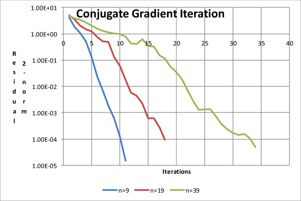
All of the discretisations converged within 40 steps. In any event the conjugate gradient method will converge in no more steps than the row/column number of the matrix, and in this case the performance of the method far exceeded that, doubtless in part to the fact that we employed a preconditioner to accelerate the solution.

As mentioned in the code comments, the method used is conjugate gradient as outlined in Gourdin and Boumahrat (2003). The method begins by computing the original residual:

$r^{\left(0\right)}=b-Ax^{\left(0\right)}$

We then solve the following equation

$Cp^{\left(0\right)}=r^{\left(0\right)}$

At this point we need to consider the conditioning matrix $C$ . It is defined as follows:

$C=TT^{t}$

where $T$ is the lower diagonal portion of $A$ . As an aside, this is an incomplete Cholesky factorization. Obviously $T^{t}$ is the upper diagonal, $A$ being symmetric. Since we have an upper diagonal solver, it would make sense to compute and invert $C$ using $T^{t}$ .

To accomplish this, we invert this to yield

$C^{-1}=\left(TT^{t}\right)^{-1}=\left(T^{t}\right)^{-1}\left(T\right)^{-1}$

We can accomplish the first term of the right hand side with the information at hand. For the second term, considering

$\left(T^{t}\right)^{-1}=\left(T^{-1}\right)^{t}$

we transpose both sides to yield

$\left(T\right)^{-1}=\left(\left(T^{t}\right)^{-1}\right)^{t}$

and substituting

$C^{-1}=\left(T^{t}\right)^{-1}\left(\left(T^{t}\right)^{-1}\right)^{t}$

We can use the factoring method to invert $T^{t}$ , then take its transpose, then multiply $\left(T^{t}\right)^{-1}$ by its transpose to yield $C^{-1}$ , which is in essence our conditioning matrix and which can be used to solve for the vector $p$ .

Returning to the algorithm, to save calculations later we define the
vector

$s=C^{-1}r$

and solving

$p^{\left(0\right)}=C^{-1}r^{\left(0\right)}$

we equate
$s^{\left(0\right)}=p^{\left(0\right)}$

We now begin our iteration for $k=1,2,3,\ldots k_{max}$ . We first compute

$\tilde{\alpha}=\frac{\left(r^{\left(k\right)}\right)^{t}s^{\left(k\right)}}{\left(p^{\left(k\right)}\right)^{t}Ap^{\left(k\right)}}$

for which purpose we developed a special subroutine. We then update our step as follows:

$x^{\left(k+1\right)}=x^{\left(k\right)}+\tilde{\alpha}p^{\left(k+1\right)}$

$r^{\left(k+1\right)}=b-Ax^{\left(k+1\right)}$

Using the conditioning matrix we developed, we compute the following

$s^{\left(k+1\right)}=C^{-1}r^{\left(k+1\right)}$

and (using a similar routine we used for $\tilde{\alpha}$ )

$\tilde{\beta}=\frac{\left(r^{\left(k+1\right)}\right)^{t}s^{k+1}}{\left(r^{\left(k\right)}\right)^{t}s^{\left(k\right)}}$

and

$\tilde{p}^{\left(k+1\right)}=s^{\left(k+1\right)}+\tilde{\beta}^{\left(k+1\right)}p^{\left(k\right)}$

From here we index $k$ and repeat the cycle until either we reach $k_{max}$ or our convergence criterion. It should be noted that the efficiency of conjugate gradient was such that, particularly at the finer discretizations, the routine spent more time generating the preconditioning matrices than it did in actually going through the cycles!

Solution Code

The solution codes were written in FORTRAN 77, and is presented below. The traditional FORTRAN column spacing got messed up in the cut and paste. Also presented is some of the code which was incorporated using the INCLUDE statement of Open WATCOM FORTRAN. The size of the grid was varied using the parameter statement at the beginning of the problem,and is generally set to 39 for the codes presented. It was varied to 9 and 19 as needed.

We should also note that the routine was run in single precision.

 c Solution of Two-Dimensional Grid Using
 c Conjugate Gradient Iteration
 c Implementation of conjugate gradient method
 c as per Gourdin and Boumahrat (2003)
 c Includes preconditioning by construction of matrix C
 c Matrix size changed via parameter statement
 include 'mpar.for'
 parameter(pi=3.141592654,istep=2000)
 c Define arrays for main array, diagonal block, off-diagonal block,
 c and solution and rhs vectors
 dimension a(nn,nn),d(n,n),c(n,n),u(nn),b(nn)
 c Define conditioning and related matrices
 dimension cond(nn,nn),t(nn,nn),tt(nn,nn)
 c Define residual vectors and norm for residual
 dimension r(nn),rold(nn),p(nn),s(nn),sold(nn),xnorm(istep)
 c Coordinate Arrays
 dimension x(n,n),y(n,n)
 c Error Vector for Final Iterate
 dimension uerr(nn)
 c Statement function to define rhs
 f(x1,y1)=-5*y1*sin(x1)*sin(2*y1)+4*sin(x1)*cos(2*y1)
 c Statement function to define closed form solution
 fexact(x1,y1)=y1*sin(x1)*sin(2*y1)
 c Write Header for Output
 write(*,*)'Conjugate Gradient Iteration to solve',
 &' two-dimensional grid'
 write(*,*)'Grid Size = ',n,' x ',n
 write(*,*)'Matrix Size ',nn,' x ',nn
 call tstamp
 c Initialise diagonal block array
 do 20 i=1,n,1
 do 20 j=1,n,1
 if(i.eq.j) then
 d(i,j)=4.
 elseif(abs(i-j).eq.1) then
 d(i,j)=-1.
 else
 d(i,j)=0.
 endif
 20 continue
 c Initialise off-diagonal block array
 do 30 i=1,n,1
 do 30 j=1,n,1
 if(i.eq.j) then
 c(i,j)=-1.
 else
 c(i,j)=0.
 endif
 30 continue
 c Compute grid spacing h
 xh=pi/float(n+1)
 c Initialise rhs
 do 60 j=1,n,1
 do 60 i=1,n,1
 x(i,j)=float(i)*xh
 y(i,j)=float(j)*xh
 ii=(j-1)*n+i
 b(ii)=-f(x(i,j),y(i,j))*xh**2
 write(*,61)i,j,ii,x(i,j),y(i,j),b(ii)
 61 format(3i5,3f10.3)
 60 continue
 c Insert block matrices into main matrix
 call blkadd(d,c,a)
 c Initialise result vector
 do 70 ii=1,nn,1
 70 u(ii)=1.0
 c Compute first residual vector, using residual vector as temporary storage
 call xmvmat(a,u,r)
 do 75 ii=1,nn,1
 r(ii)=b(ii)-r(ii)
 75 continue
 c Construct upper triangular matrix tt by stripping lower diagonal portion of
 c matrix a
 do 76 ii=1,nn,1
 do 76 jj=1,nn,1
 if(jj-ii)78,77,77
 77 tt(ii,jj)=a(ii,jj)
 goto 76
 78 tt(ii,jj)=0.0
 76 continue
 c Invert upper triangular matrix tt by factorisation method
 call uminv(tt)
 c Construct inverted matrix t by transposing inverted matrix tt
 call trnspz(tt,t)
 c Multiply t by tt to obtain preconditioning matrix c (which is actually
 c c**(-1))
 call xmvmul(tt,t,cond)
 c Compute initial vector p by multiplying cond (inverse of c) by residual
 call xmvmat(cond,r,p)
 c Set initial vector s to p
 do 79 ii=1,nn,1
 79 s(ii)=p(ii)
 do 80 kk=1,istep,1
 c set old values of vectors r and s
 do 190 ii=1,nn,1
 rold(ii)=r(ii)
 190 sold(ii)=s(ii)
 c Compute alpha for each step
 alpha1=alpha(a,p,r,s)
 c Update value of u
 do 181 ii=1,nn,1
 181 u(ii)=u(ii)+alpha1*p(ii)
 c Update residual for each step r = b-Au
 call xmvmat(a,u,r)
 do 82 ii=1,nn,1
 r(ii)=b(ii)-r(ii)
 82 continue
 c Update vector s
 call xmvmat(cond,r,s)
 c Compute value of beta for each step
 beta1=beta(r,rold,s,sold)
 c Update value of p vector
 do 195 ii=1,nn,1
 195 p(ii)=s(ii)+beta1*p(ii)
 c Invoke function to compute Euclidean norm of residual
 c Kicks the iteration out once tolerance is reached
 xnorm(kk)=vnorm(r,nn)
 if(xnorm(kk).lt.1.0e-04)goto 83
 write(*,*)kk,xnorm(kk)
 80 continue
 83 continue
 do 90 j=1,n,1
 do 90 i=1,n,1
 ii=(j-1)*n+i
 uerr(ii)=fexact(x(i,j),y(i,j))-u(ii)
 90 continue
 uerrf=vnorm(uerr,nn)
 write(*,*)'Number of iterations = ',kk
 write(*,*)'Euclidean norm for final error =',uerrf
 open(2,file='m5610p1d.csv')
 if(kk.gt.istep)kk=istep
 do 40 ii=1,kk,1
 write(2,50)ii,xnorm(ii)
 50 format(i5,1h,,e15.5)
 40 continue
 close(2)
 stop
 end

c Subroutine to insert nxn blocks into n**2xn**2 array
 c Assumes all diagonal blocks are the same
 c Assumes all off-diagonal blocks (upper and lower) are the same
 c Assigns zero values elsewhere in the array
 subroutine blkadd(d,c,a)
 include 'm5610par.for'
 dimension a(nn,nn),d(n,n),c(n,n)
 c Insert blocks into array
 do 20 ii=1,n,1
 do 20 jj=1,n,1
 c Determine row and column index in master array for corner of block
 ic=(ii-1)*n+1
 jc=(jj-1)*n+1
 do 30 i=1,n,1
 do 30 j=1,n,1
 iii=ic+i-1
 jjj=jc+j-1
 if(ii.eq.jj)then
 a(iii,jjj)=d(i,j)
 elseif(abs(ii-jj).eq.1)then
 a(iii,jjj)=c(i,j)
 else
 a(iii,jjj)=0.
 endif
 30 continue
 20 continue
 return
 end

c Subroutine to multiply a nn x nn matrix with an nn vector
 c a is the nn x nn square matrix
 c b is the nn vector
 c c is the result
 c nn is the matrix and vector size
 c Result is obviously an nn vector
 c Routine loosely based on Gennaro (1965)
 subroutine xmvmat(a,b,c)
 include 'm5610par.for'
 dimension a(nn,nn),b(nn),c(nn)
 do 20 i=1,nn,1
 c(i)=0.0
 do 20 l=1,nn,1
 20 c(i)=c(i)+a(i,l)*b(l)
 return
 end

c Subroutine to multiply a nn x nn matrix with another nn x nn matrix
 c a is the first nn x nn square matrix
 c b is the second nn x nn matrix
 c c is the result
 c nn is the matrix size
 c Result is obviously an nn x nn matrix
 c Routine based on Gennaro (1965)
 subroutine xmvmul(a,b,c)
 include 'm5610par.for'
 dimension a(nn,nn),b(nn,nn),c(nn,nn)
 do 20 i=1,nn,1
 write(*,*)'Multiplying Row ',i
 do 20 j=1,nn,1
 c(i,j)=0.0
 do 20 l=1,nn,1
 20 c(i,j)=c(i,j)+a(i,l)*b(l,j)
 return
 end

c Subroutine to invert a mm x mm upper triangular matrix using factor method
 c u is input and output matrix
 c t is result matrix, written back into the output matrix
 c mm is matrix size
 c Result overwrites original matrix
 c Based on Gennaro (1965)
 subroutine uminv(u)
 include 'm5610par.for'
 dimension u(nn,nn),t(nn,nn)
 c Zero all entries in matrix t except for diagonals, which are the reciprocals
 c of the diagonals of the orignal matrix
 do 20 i=1,nn,1
 do 20 j=1,nn,1
 if(i-j)11,10,11
 10 t(i,j)=1.0/u(i,j)
 goto 20
 11 t(i,j)=0.0
 20 continue
 c Compute strictly upper triangular entries of inverted matrix
 do 40 i=1,nn,1
 write(*,*)'Inverting Row ',i
 do 40 j=1,nn,1
 if(j-i)40,40,31
 31 l=j-1
 do 41 k=i,l,1
 t(i,j)=t(i,j)-t(i,k)*u(k,j)/u(j,j)
 41 continue
 40 continue
 c Write back result into original input matrix
 do 50 i=1,nn,1
 do 50 j=1,nn,1
 50 u(i,j)=t(i,j)
 return
 end

c Function to compute Euclidean norms of vector
 function vnorm(V,no)
 dimension V(no)
 znorm=0.
 do 100 ia=1,no,1
 100 znorm=znorm+V(ia)**2
 vnorm=sqrt(znorm)
 return
 end

c Function to determine scalar multiplier alpha for conjugate gradient method
 c Function returns a scalar which is multiplied by residual vector
 c Function uses subroutine xmvmat to multiply matrix A by residual
 c A is main matrix
 c r is residual vector
 c nn is size of matrix/vector
 c rgrad is scalar multiplier for gradient method
 function alpha(a,p,r,s)
 include 'm5610par.for'
 dimension a(nn,nn),r(nn),pt(nn),p(nn),s(nn)
 c Compute dot product of r and s for numerator
 rnumer=0.0
 do 10 ii=1,nn,1
 rnumer=rnumer+r(ii)*s(ii)
 10 continue
 c Compute matrix product of A * p
 call xmvmat(a,p,pt)
 c Premultiply matrix product by transpose of p vector for denominator
 rdenom=0.0
 do 20 ii=1,nn,1
 rdenom=rdenom+p(ii)*pt(ii)
 20 continue
 alpha = rnumer/rdenom
 return
 end

c Function to determine scalar multiplier beta for conjugate gradient method
 c Function returns a scalar which is multiplied by p vector
 c r,s are vectors is residual vector
 c nn is size of matrix/vector
 c rgrad is scalar multiplier for gradient method
 function beta(r,rold,s,sold)
 include 'm5610par.for'
 dimension r(nn),rold(nn),s(nn),sold(nn)
 c Compute dot product for numerator
 rnumer=0.0
 do 10 ii=1,nn,1
 rnumer=rnumer+r(ii)*s(ii)
 10 continue
 c Compute dot product for denominator
 rdenom=0.0
 do 20 ii=1,nn,1
 rdenom=rdenom+rold(ii)*sold(ii)
 20 continue
 beta = rnumer/rdenom
 return
 end

c Subroutine to transpose a matrix
 c Adapted from Carnahan, Luther and Wilkes (1969)
 subroutine trnspz(a,at)
 include 'm5610par.for'
 dimension a(nn,nn),at(nn,nn)
 do 14 ii=1,nn,1
 do 14 jj=1,nn,1
 14 at(jj,ii)=a(ii,jj)
 return
 end

include 'tstamp.for'

Included Routines

tstamp.for calls a OPEN WATCOM function and time stamps the output.
mpar.for sets the parameter statements and is shown below.

 parameter(n=39,nn=n*n)

References

Carnahan, B., Luther, H.A., and Wilkes, J.O. (1969) Applied Numerical Methods. New York: Wiley.
Gennaro, J.J. (1965) Computer Methods in Solid Mechanics. New York: Macmillan.
Gourdin, A., and Boumahrat, M. (2003) Applied Numerical Methods. New Delhi: Prentice-Hall India.