The General Form of Circular Motion for Particle Kinematics, and an Example with Time-Varying Rotational Velocity

In the last post we looked at straight line motion for particle kinematics, and in another post we looked at constant angular velocity results. In this post we will a)consider the general form of the equations for circular motion and b)look at an example of linear rotational acceleration.

General Form

We start by generalising the equations for circular motion by saying that, instead of the angle θ of the position vector (which still has a constant radius r with the centre of rotation) having a constant angular velocity and thus being ωt, we say that it is a general function of time θ(t). Formulating them in a similar manner to this post, the position, velocity and acceleration vector can be written thus:

$r(t)=r\left(\cos(\theta(t))i+\sin(\theta(t))j\right)$ (1)

${\frac{d}{dt}}r(t)=-r\left({\frac{d}{dt}}\theta(t)\right)\left(\sin(\theta(t))i-\cos(\theta(t))j\right)$ (2)

${\frac{d^{2}}{d{t}^{2}}}r(t)=-r\left(\left({\frac{d^{2}}{d{t}^{2}}}\theta(t)\right)\sin(\theta(t))i-\left({\frac{d^{2}}{d{t}^{2}}}\theta(t)\right)\cos(\theta(t))j+\left({\frac{d}{dt}}\theta(t)\right)^{2}\cos(\theta(t))i+\left({\frac{d}{dt}}\theta(t)\right)^{2}\sin(\theta(t))j\right)$ (3)

Although these at first glance these don’t seem to be very useful, once we substitute a function for θ(t) their value will become apparent.

Example

The example used here is taken from Theoretical Mechanics – A Short Course -Targ, although the vector approach we will take is different from theirs. The problem is stated as follows (with some modifications):

A train starts moving from rest with uniform acceleration along a curve of radius r = 800 m and reaches a velocity v₂ = 36 km/h after travelling a distance s₂ = 600 m. Determine the velocity…of the train at the middle of this distance.

We define the middle point as s₁. We need to do two things at the start. The first is to determine the angle θ of the train at Point 2. This is simply

$\theta_2 = \frac{s_2}{r}$ (4)

Simple substitution yields θ₂ = 0.75 radians = 43 degrees.

The second is to establish the function θ(t). Since it is uniform acceleration with respect to time, it can be established as follows:

$\theta(t) = \alpha t \times t = \alpha t^2$ (5)

where α is the acceleration coefficient, which is in units of sec^-2 and is constant. Substituting this results into Equations (1), (2) and (3) yields the following:

$r(t)=r\left (\cos(\alpha\,{t}^{2})i+\sin(\alpha\,{t}^{2})j\right )$ (6)

${\frac {d}{dt}}r(t)=r\left (-2\,\sin(\alpha\,{t}^{2})\alpha\,ti+2\,\cos(\alpha\,{t}^{2})\alpha\,tj\right )$ (7)

${\frac {d^{2}}{d{t}^{2}}}r(t)=r\left (-4\,\cos(\alpha\,{t}^{2}){\alpha}^{2}{t}^{2}i-2\,\sin(\alpha\,{t}^{2})\alpha\,i-4\,\sin(\alpha\,{t}^{2}){\alpha}^{2}{t}^{2}j+2\,\cos(\alpha\,{t}^{2})\alpha\,j\right )$ (8)

At this point we need to determine the values of α and t at the boundary condition point 2, where we know s₂ and the scalar velocity v₂. We do this by setting the scalar magnitude of the right hand side of Equation (7) to the final scalar velocity v₂. Going through the algebra, we end up with

${\it v_2}=2\,\alpha\,tr$ (9)

At this point we need to note two things:

$\alpha=\frac{\theta_2}{t^2}$ (10) (from Equation (5))
$r = \frac{s_2}{\theta_2}$ (11) (from Equation (4))

Putting these together with Equation (9) yields

$t = 2\,{\frac {{\it s_2}}{{\it v_2}}}$ (12)

and from

${\it v_2^2}=4\,{\alpha\,{\it s_2}\,r}$ (13)

we have

$\alpha=1/4\,{\frac {{{\it v_2}}^{2}}{{\it s_2}\,r}}$ (14)

Substituting, we have α = 27/40000 sec^-2 and t = 100/3 sec.

At this point we should note that Equation (13) is valid for any combination of velocity and position. For the midpoint position 1, the velocity can be computed from the equation

$v_1 = 2 \sqrt{\alpha s_1 r}$ (15)

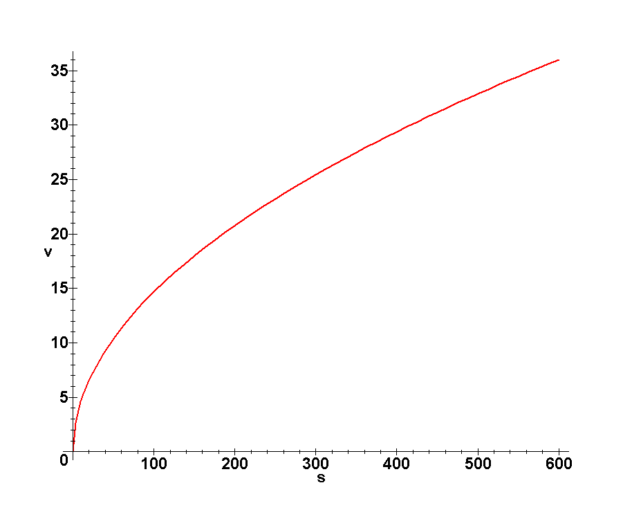
Substituting the values of α and r and the midpoint s₁ = 300 m, v₁ = 25.5 m/sec. It is worth noting that in Theoretical Mechanics – A Short Course -Targ the final answer is different, but earlier it is stated that the midpoint velocity is the final velocity divided by the square root of 2, which gives the same result as we have.

A plot of Equation (13) for velocity as a function of distance is shown below.