Fluid mechanics courses frequently start by regaling their students with equations in these forms:
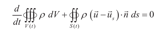
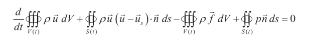

Although these equations are true and certainly useful in proper context, for students starting out they don’t make a very gentle climb to understanding. In this post we’re going to look at an example which is solved in a simpler fashion and should emphasise the importance of the conservation of momentum in fluid mechanics problems. In some ways conservation of momentum is more important in fluid mechanics than it is in solid mechanics; it is the reason why moving fluids exert a force on an object in their path. We have an experimental example of this in Fluid Mechanics Laboratory Video: Propeller and Momentum Theory Experiment, and the theory behind it is discussed in Chet’s Propellers: How Did They Work? We’ll start by presenting that theory in a way that is more general.
The Basic Theory
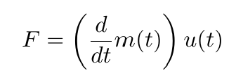
A more basic statement of the conservation of momentum (Equation (2)) is
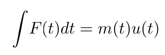
(4)
where
- F(t) = force exerted by a fluid
- t = time
- m(t) = mass as a function of time
- u(t) = velocity in the x-direction
The last deserves some explanation. In Equations (1-3), u is a velocity vector. For one-dimensional problems u(t) is the velocity in the x-direction (the one-dimension in question.) With three-dimensional problems, if we stick with a Cartesian scalar scheme, v(t) is the velocity in the y-direction and w(t) is the velocity in the z-direction. Careful examination of Equation (2) will confirm that momentum is a vector quantity, as is the case with solid mechanics.
Differentiating Equation (4),

(5)
For the steady state condition,
(6)
The Example Problem
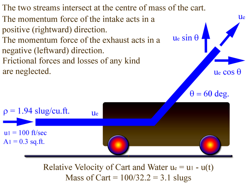
The example problem we’re looking at is taken from Fox and McDonald (1973) and is shown in Figure 1.

The water jet is basically pushing the cart from rest to the right with a constant flow rate. The water stream curves through the cart and exits on the “back side” of the cart as shown. While the original posits the equations in a form similar to Equations (1) and (2), since we will only consider the effects in the x-axis (the cart is constrained from moving in the y-axis as long as the forces in that direction are downward) we will use a simpler form of these equations.
For the steady state problems we have here, the continuity (conservation of mass flow) equation is
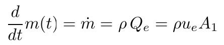
(7)
where
mass flow, slugs/sec
density, slugs/ft3
relative velocity of the flow stream and the cart, ft/sec
volume flow rate of stream, ft3/sec
cross-sectional area of flow stream, ft2
The momentum equation–which leads to the force acting on the cart by the stream–can be stated thus

(8, from Equations (6) and (7))
where
force the stream exerts on the cart, lbs.
reaction of the cart assuming either the cart is stationary or constrained to move at a given velocity, lbs.
angle of the vane, radians or degrees
The key is to understand that the momentum induced force depends not on the absolute velocity of the flow stream but the relative velocity of the flow to that of the cart, defined as
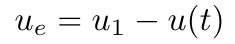
(9)
where 
At this point, let us introduce some solid mechanics, in this case dynamics in one dimension. We know the magnitude of the force on the cart assuming we know the relative velocity of the cart and the flow from Equation (8). Using d’Alembert’s method (described in Theoretical Mechanics by M. Movnin; A. Izrayelit, and applied in the post An Example of Kinetics of Circular Motion) we can turn this into a pseudostatic problem by including the inertial term in this way:
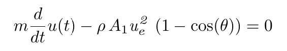
(10)
Note that the inertial term is the first derivative of the velocity rather than the second derivative of the displacement; these are the same. Expanding this using Equation (9),
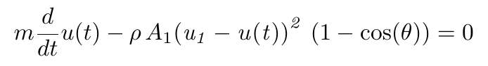
(11)
At this point we search for a solution method for the problem. Fox and McDonald (1973) suggest using the method of separation of variables, but some explanation of this is in order. According to Bronshtein and Semendyayev (1971), if we have a differential equation of the form
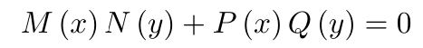
(12)
we can write it thus
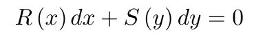
(13)
by dividing through in this way
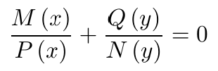
(14)
and integrating to

(15)
Equation (11) can be written in the form of Equation (14) by substituting
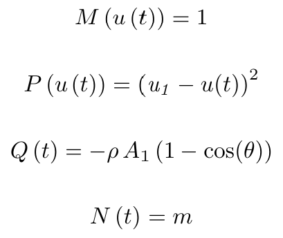
(16)
Doing this yields

(17)
Applying Equation (15) (integrating,) we obtain
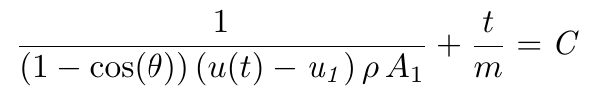
(18)
The initial conditions are u(0)=0 at t=0. Substituting these and solving first for C and then u(t), we have at last
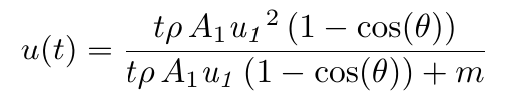
(19)
Normalizing this for u1 and rearranging terms brings us
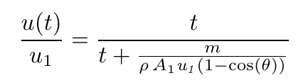
(20)
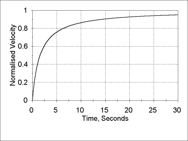
and substituting the parameters shown in Figure 1 gives the numerical result
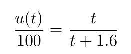
(21)
This is plotted in Figure 2. It makes sense that, as the velocity of the cart approaches the velocity of the fluid stream, the increase of the velocity will decrease to zero.
References not Linked in Narrative
- Bronshtein, I.N., and Semendyayev, K.A. (1971) A Guide-Book to Mathematics. Frankfurt/Main: Verlag Harri Deutsch
- Fox, R.W., and McDonald, A.T. (1973) Introduction of Fluid Mechanics. New York: John Wiley & Sons, Inc.
- Swafford, T.W. (2011) Computational Fluid Dynamics: An Introduction to the Fluid Dynamics Equations and Formulations for Numerical Solutions. Unpublished Notes.
