
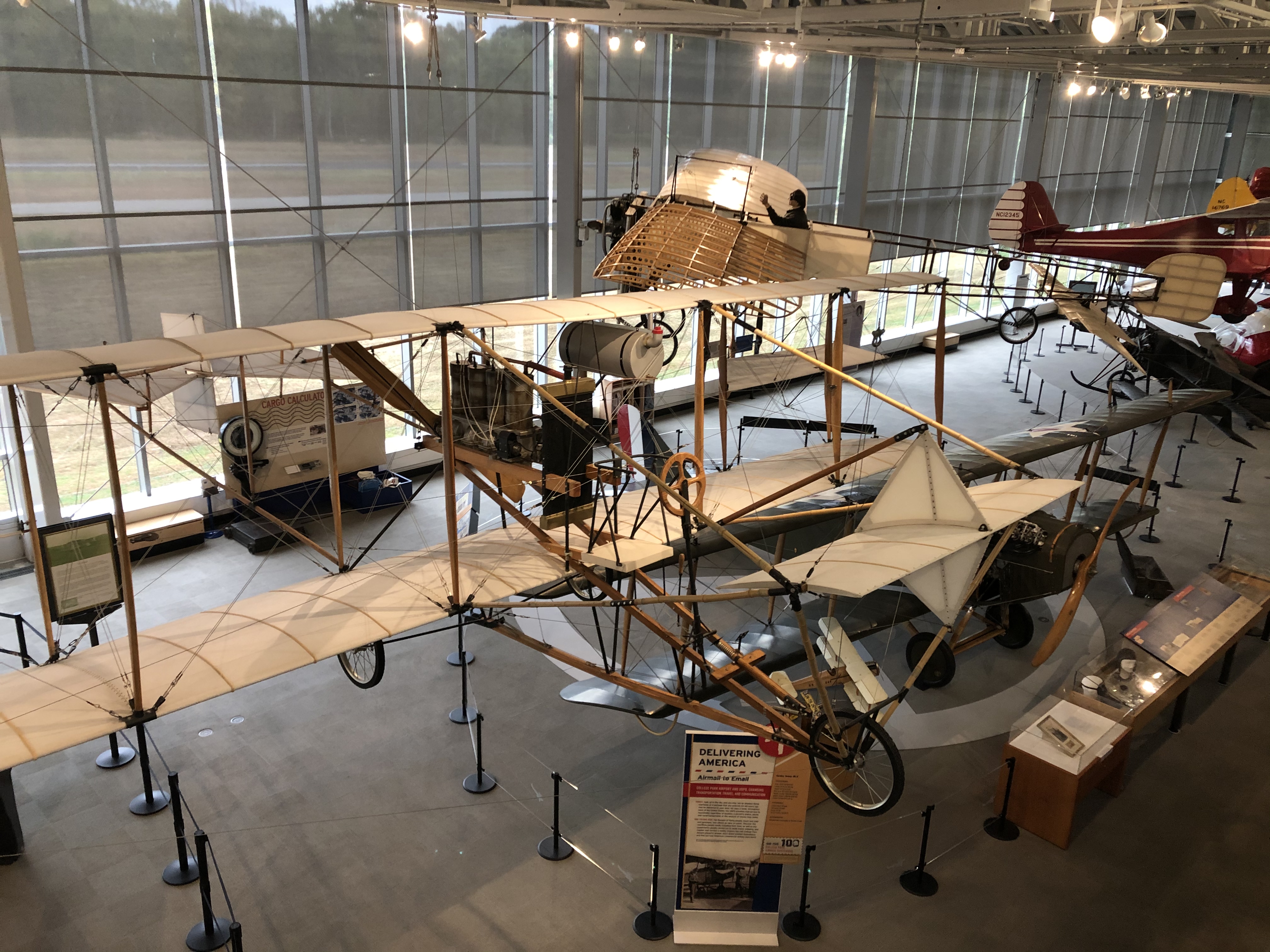
All of Chet’s planes–and those of the people around him–were propeller-driven aircraft. With the advent of jet aircraft after World War II, it seemed that propeller-driven craft were relegated to private use or “puddle jumpers” for commercial aviation. But the advent of drone technology has put propellers back into the spotlight, although, like the auto-gyros of Chet’s day and the helicopters that succeeded them, it applies them in a different way. But the principles are the same. (In reverse, it’s the same technology that’s used with wind turbines.)
How Aircraft Stay Aloft

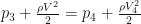
Let’s start by looking at the diagram on the right, the top panel. It’s really a matter of static and/or dynamic equilibrium: as the propeller or jet engine produces thrust, the plane moves forward, inducing upward lift in the wings to overcome the downward force of gravity. The thrust also overcomes the drag which is inevitable with bodies moving through the air. By definition the thrust must be greater than the drag for forward motion of the aircraft, and the lift must be equal to the force of gravity to maintain level flight (that relationship changes as the aircraft pitches, rolls and yaws.)
Concerning the pitch, if we look at the second panel, as the aircraft pitches upward, the component of the gravity in the direction of thrust and drag increases. The lift does not necessarily increase, so one would expect the aircraft to slow down with a constant thrust as it ascends, which in fact they do. The opposite effect is shown in the third panel, which shows a descending aircraft.
The last panel links conventional propeller-driven aircraft of Chet’s day and now with drones, as it shows an extreme upward pitch. With a drone the angle between the horizontal and the thrust becomes 90 degrees or nearly so. When the drone is stationary the drag is zero as the velocity is zero; for the drone to maintain a constant altitude the thrust and gravity must be equal. To move the drone up and down the thrust can be varied. Additional sources of thrust must be used to move the drone from side to side.
For more information on the airfoils that produce lift and related topics, please see our monograph Wind Tunnel Testing.
The Basics of Propellers
Propellers antedate aircraft; they first find themselves on marine craft, something which Chet, his ancestors and descendants were well familiar with. It is the reason why someone like Froude, who has been mentioned elsewhere, developed the momentum theory for propeller operation, which we will discuss later. An example of a propeller on a ship, in this case a steam yacht, is shown below.

In any case some of the basic terminology of aircraft propellers is shown below.

Note that, as the sections are taken further out from the centre, the blade’s orientation changes. This is to maintain a constant angle of attack from centre to edge of the blades due to the linear increase of the speed as the distance increases from the centre. This innovation was done by the Wright brothers and was crucial in their successful pioneering flights.


Basically propellers act as a screw in the fluid they’re immersed in, driving the ship or plane forward in a similar fashion as a screw does in a solid. (I can remember that, during my yachting years, the ships’ propellers were referred to as “screws.”) If the fluid is incompressible and everything is “efficient,” then the screw will propel the ship or plane like its solid counterpart. Unfortunately that seldom happens, so there is slip, and the actual travel per revolution of the propeller is less than ideal.

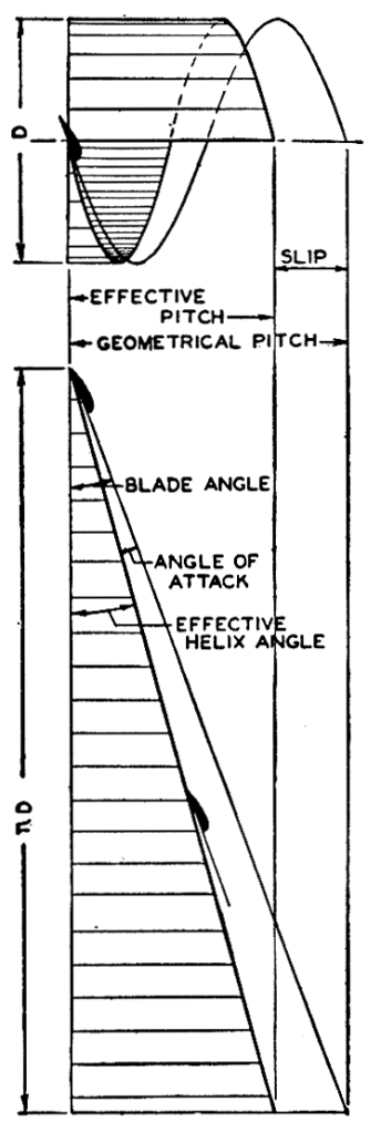
The interaction between the advancing propeller and the air it travels through is shown at the right. A propeller is basically an airfoil, as should be evident by looking at these diagrams. Airfoils, as discussed in Wind Tunnel Testing, generate lift by passing the air over them, generating differential pressure between the upper surface and the lower surface. Drag is an inevitable result of a body passing through a viscous fluid (and if the airfoil is not symmetric about the chord, an inviscid one too.)
Let’s start by assuming that the propeller profile is not symmetric (and most are this way.) If there is no slip, the angle of attack between the propeller blade and the airflow produced by the propeller is zero, and the blade and effective helix angles are the same.
As slip increases, the angle of attack increases, which means that we have to watch for stall in the design of the propeller. When the craft isn’t moving forward at all, the blade angle and angle of attack are the same.
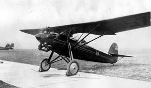
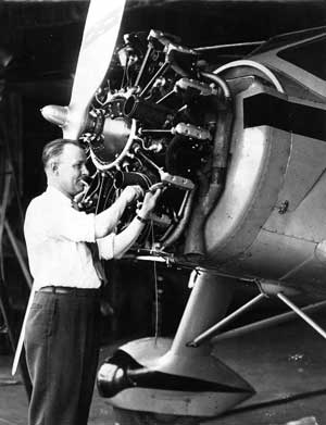
In Chet’s day, the way you got to the last state was to put chocks under the wheels and run the engine and propeller, as you can see below. Now producing thrust against a motionless craft is part of the design objective. It’s not the most efficient use of propeller technology, but it’s useful and it works, especially now with the advances in electric motors and batteries and control systems. It’s a good example of how applications of technology aren’t always the most efficient but produce desirable results.
Momentum Theory and Propeller Performance
With the preliminaries out of the way, we’ll get to the heart of the matter: how do we estimate the performance of propellers? The “classic” way to do this is momentum theory, which was first derived by Froude. There are other theories out there (blade-element theory comes to mind) but momentum theory, crude as it is, is a good place to start. The derivation we present is a standard derivation; this presentation is based on Streeter with some modification.
Let us start with presenting a diagram of the system and its control volume, shown below.

We’ll also make a few assumptions:
- The fluid is inviscid, so Bernoulli’s Equation can be used.
- The fluid is incompressible. This may seem unbelievable with air, but the pressure differences–and by extension the density differences–make this assumption possible. (After all, we did say this theory was crude…)
- The fluid velocity is uniform at any x-axis point in the control volume, similar to the assumption we make with piping
- As it passes across the propeller, the fluid’s pressure changes but its velocity does not.
- The shape of the control volume, but we’ll justify that in a minute
That being the case, there are two ways we can analyse this. The first is to use momentum theory of fluids. A detained discussion of this is beyond the scope of this presentation, but it can be shown that the net force (thrust) exerted by the control volume on the surrounding fluid is

since

and

The nomenclature is at the end.
Another way is to note that the thrust is, by static equilibrium, equal to the differential pressure across the propeller times the area the propeller sweeps during rotation, or

we can equate Equations (1) and (4) yield

To arrive at values for the two pressures, we turn to Bernoulli’s Equation, which we have discussed elsewhere. Dropping the gravity term out entirely from our considerations, from point 1 to 2 we have

and from point 3 to 4,
Combining the two, and assuming that both 


Equating the left hand side of Equation (5) with the right hand side of Equation (8) and rearranging, we have at last

From this the fluid velocity at the propeller is the average of the velocities a the boundary of the control volume. This is a nice result; some professors will confidently assert that it is “intuitively obvious,” but we’ll try to spare you from such conceit.
Power and Energy Losses
The useful work (power) done by the propeller in moving the aircraft forward is given by the equation

Obviously all of the energy put into rotating the propeller does not end up moving the aircraft forward; the total power input is given by the equation

The efficiency, i.e., the ratio of the useful power to the total power input, is thus

Reducing the Control Volume
Up until now we’ve assumed a control volume which goes from Points 1 to 4 in the diagram above. We do this because it’s usually easier to measure the velocities 

The usefulness of this will become apparent.
Test Stand Case and Calculations
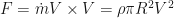
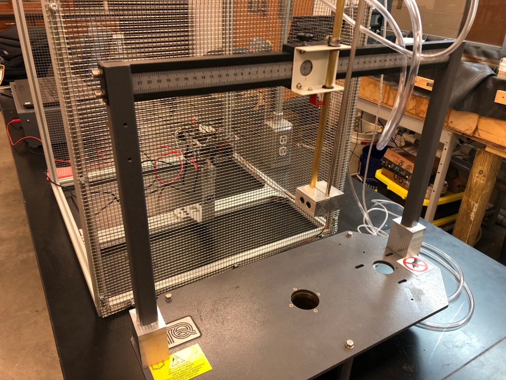
We start with a test stand, shown below.


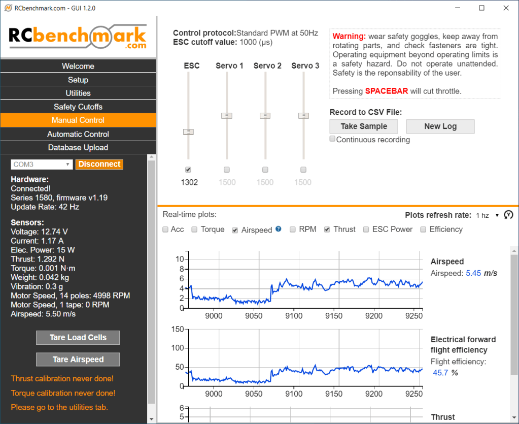
At this point we’ll use the traverse to record a series of velocity readings across the output of the propeller. There is more than one way to do this; the method we’ll employ divides up the area facing the propeller into annuli as follows:
Let’s use the centimetres as an index. With apologies to my fellow FORTRAN programmers, that makes the centre index zero. Using the tall grid marks as the points where we take our data, the area of the annulus around the data point is given by the equation

The only exception to this is the centre circle, whose area is

Thus, for each circle/annulus, Equation (13) becomes

The areas are obviously in square centimetres and unfortunately will have to be converted to square meters to use.
Now consider the sample case. The recorded positions of the Pitot-static tube and the velocity are given as follows:
| Distance from Centre, cm | Air Speed, m/sec |
| 12 | 1.25 |
| 10 | 2 |
| 8 | 3.8 |
| 6 | 6.8 |
| 4 | 7.7 |
| 2 | 6 |
| 0 | 4 |
| -2 | 6.7 |
| -4 | 7.8 |
| -6 | 6.6 |
| -8 | 4.2 |
| -10 | 1.8 |
| -12 | 1.4 |
At this point we need to do three things: a) average the pairs of air speeds for the radii, b) compute the areas of the annuli, and c) compute the thrust on the annulus using Equation (13). This is done in the table below
| Distance from Centre, cm | Average Air Speed, m/sec | Annulus Cross-Section Area, sq. cm. | Thrust from Equation (16), N |
| 12 | 1.325 | 150.8 | 0.032 |
| 10 | 1.9 | 125.7 | 0.054 |
| 8 | 4 | 100.5 | 0.194 |
| 6 | 6.7 | 75.4 | 0.407 |
| 4 | 7.75 | 50.2 | 0.363 |
| 2 | 6.35 | 25.1 | 0.122 |
| 0 | 4 | 3.14 | 0.006 |
The thrusts are then summed to 1.18 N, which is within 9% of the instrumented total.
Acknowledgements
I would like to thank Dr. Kidambi Sreenivas and Mr. Jacob Jenkins of the University of Tennessee at Chattanooga, without whose efforts this experiment would not have come into being.
Nomenclature


References
- Elger, D.F., LeBret, B.A., Crowe, C.T. and Roberson, J.A. (2016) Engineering Fluid Mechanics. Eleventh Edition. Hoboken, NJ: John Wiley & Sons Inc.
- Hibbler, R.C. (2018) Fluid Mechanics. Second Edition. New York: Pearson.
- Lusk, H.F. (1940) General Aeronautics. New York: Ronald Press Company
- Jordanoff, A. (1936) Your Wings. New York: Funk and Wagnalls Company
- Streeter, V.L. (1966) Fluid Mechanics. Fourth Edition. New York: McGraw-Hill Book Company
- Vennard, J.K. 1940) Elementary Fluid Mechanics. New York: John Wiley & Sons Inc.
- Wood, K.D. (1935) Technical Aerodynamics. New York: McGraw-Hill Book Company
