Our main fluid mechanics laboratory page is here.
Scroll down for the procedure. Other resources relating to this laboratory is here:
- Background Material (important to understand the topic)
- Helpful Material
- Compressible Flow Through Nozzles. A look at flow with compressible fluids such as air.
- Getting the Reynolds Number Right. Messing up this calculation is an error I see too often; this should help.
- Valve Loss Study. Although this was with compressible fluids, the basic concepts are the same.
- “I Need to Find the Way”. Fluid Mechanics can be a stinker, as one Turk found out the hard way.
Procedure
Note: depending upon the instructor, this lab can be done in one or two parts. If it is done in two parts, the Moody Chart correlation is done separately from the rest. You need to read your instructor’s directions to know whether this is the case or not. Failure to do so can result in extra work. In either case you need to download the Data Spreadsheet for Fluid Flow in Pipes, Losses, Flow Metering and Moody Chart Experiment. There’s a lot of data to be taken in this experiment; it will be helpful in organising that data.
Introduction
In many engineering applications, determining the flow rate of a fluid in a closed channel is very important. Flow meters break down into three types:
- “Classical” flow meters which use velocity changes and energy losses in the fluid to estimate the flow;
- Mechanical flow meters such as the rotameter which estimate the flow using other means; and
- Electronic flow meters which use various methods to estimate the flow. These have digital output, which can be read either directly from the device, through a data acquisition system, or both.
In this experiment we will be dealing with all three types of flow meters. Although classical flow meters are not as widespread as they once were, they are an important topic to demonstrate energy losses in fluid flow; see Fluid Flow in Pipes, Losses and Flow Metering (instructor’s handout) for more information.
Additionally, energy losses must be considered for the entire system. Pipes, elbows, contractions, enlargements and valves all contribute to energy loss in a piping system and must be analyzed. Pipe losses are major energy losses, while all others are usually minor. A valve, such as a gate valve, has losses that are a function of both the amount the valve is open and the flow rate that passes through the valve. These losses are studied in this lab in two ways:
- Pipe losses in a straight pipe; and
- Minor losses in a portion of pipe with obstacles such as pipe elbows and the Rotameter itself.
Objective
The objective of this laboratory is fourfold, using a digital flow meter as the “reference” flow:
- To calibrate each of the flow meters in the hydraulic flow bench system. This will involve determining the coefficient of discharge for each classical flow meter (the two orifices, flow nozzle, and venturi flow meters;)
- To directly compare the flow measurement of a mechanical flow meter (the Rotameter) with the digital flow meter;
- To study head losses by comparing the losses in a portion of pipe with obstacles with the equivalent length of straight pipe; and
- To study losses in a straight pipe, comparing them to those predicted by the Moody Chart. This may be done separately from the rest of the experiment.
Basic Theory of “Classical” Flow Meters and Losses in Piping Systems
The theory behind classical flow meters is discussed in Fluid Flow in Pipes, Losses and Flow Metering (instructor’s handout.)
Pipe Losses
Pipe losses are estimated using the Moody Chart; this is explained in Fluid Flow in Pipes, Losses and Flow Metering (instructor’s handout.) This is also explained in your fluid mechanics textbook. There are also formulas which replicate parts of the Moody Chart which are easier to use in a spreadsheet; these are also in both Fluid Flow in Pipes, Losses and Flow Metering (instructor’s handout) and in your textbook.
Minor Losses
Minor losses take place in common pipe fittings such as tees, elbows, etc. For this experiment a portion of the flow bench has two pressure ports which connect to a digital manometer. The portion has four (4) elbows and the Rotameter. The loss coefficient K (discussed in Fluid Flow in Pipes, Losses and Flow Metering (instructor’s handout)) is computed for this portion of the flow bench, and compared with a comparable section of straight pipe to see the effects of the minor losses. The theory is the same as that of classic or classical flow meters, but the way the loss coefficient is handled is different.
Apparatus
The entire experiment is performed on the flow bench, which is shown below.

The pump (and its controls) is to the right of the reservoir (the white barrel in the front of the photo.) Pressurized water enters on the right side of the end of the table and flows down a series of pipes on the right side of the table. On that side is the digital flow meter and three of the four classical flow meters: Orifice #1, the Flow Nozzle and the Venturi. A sketch of the system with the valve numbers and other information is below.
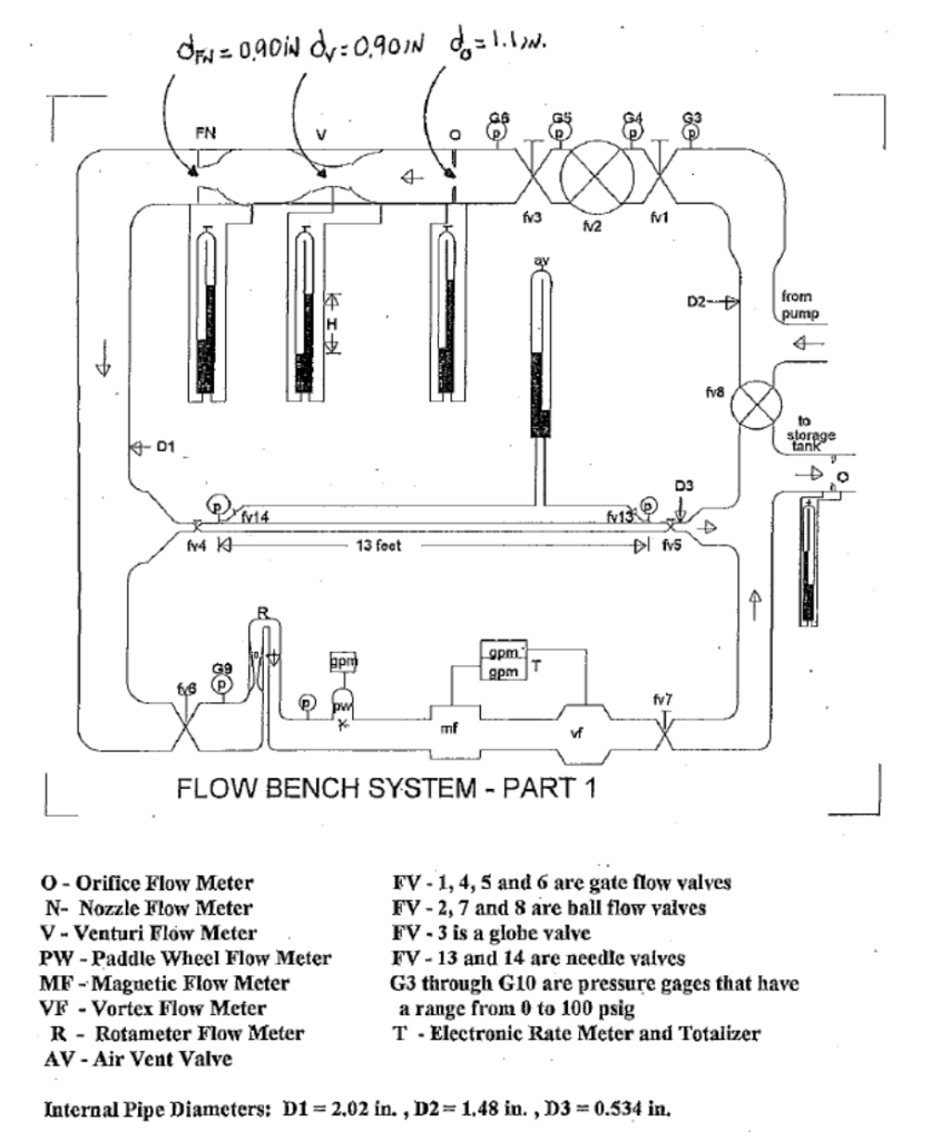
Notes on the chart:
- The electronic flow meters PW, MF, VF and the valves FV 6 have been eliminated from the flow bench.
- The valves FV 2, and FV 3 are open at all times.
- The electronic flow meter is where FV 1 used to be.
- The manometers for O, N, V and on either side of R are digital.
- Orifice #2 is on the far right hand side of the chart; it is a conventional fluid manometer.
- The distance between the pressure ports at FV 4 and FV 5 is actually 12′.
- The minor loss region is around the rotameter R; the digital manometer for this region is connected to the two pressure ports on either side of it.
The water courses around the far end of the table. At this point there are two options for the flow, depending upon what is being done.
- Flow Valves 4 (FV 4) is closed, and Flow Valve 7 (FV 7) is open. This is the way the flow meter calibration and the gate valve correlation are done.
- Flow Valves 4 is open and Flow Valve 7 is closed. This is the way the Moody Chart pipe loss correlation is done. This may be done separately from the rest of the experiment.
The water returns to the reservoir as follows:
- The water for the conventional flow meters (and that includes Orifice #2) can return to the reservoir if either or both Valves #4 and #7 are open. For our purposes, we will close Valve #7 to collect data for these flow meters.
- The water for the Rotameter and the Minor Loss area can return to the reservoir if Valve #4 is closed and Valve #7 is open. Doing this allows the same flow through the digital flow meter and the Rotameter, making comparison between the two valid.
- The water for the Moody Chart portion of the experiment can return to the reservoir if Valve #4 is open and Valve #7 is closed. This makes the flow recorded by the digital flowmeter the same as is flowing through the pipe.

The reference flow meter for all parts of this experiment is the digital flow meter at the “head” of the flow bench, shown above. That reference will measure the flow at each flow rate, against which you will use the data from the manometers to compute the coefficient of discharge for each flow meter at each data point. It reads the flow in gallons per minute.
The diameters of the various components are as follows (in case they’re hard to read on the chart):
| Flow Device | d1, inches | d2, inches |
| Orifice #1 | 1.48 | 1.10 |
| Orifice #2 | 2.02 | 1.25 |
| Flow Nozzle | 1.48 | 0.90 |
| Venturi | 1.48 | 0.90 |
Also dimensions are given for the following:
- The Moody Chart portion of the experiment is run through a 12’ long stretch of ½” Type L copper tubing, I.D. = 0.545”. Estimates of the roughness can be found in your fluid mechanics textbook.
- For Rotameter/Minor Loss Experiment Area: the water flows through approximately 4’ of pipe, elbows and the Rotameter between the two ports of the digital manometer. The pipe inside diameter in this area (obviously excluding the Rotameter and the elbows) is approximately 1”. For equivalent length purposes assume the PVC pipe is smooth.
One more important note: students may become confused when they see negative head differentials across the digital flow meters or notice differences in terms of which fluid column is higher for a given fluid manometer. These are strictly a function of how the manometer is hooked up and should be ignored for data collection purposes. Also, for the fluid/analog manometer (Orifice #2,) the absolute height of the water columns is not what you’re trying to measure; you need to measure the difference in heights. This difference is the only thing that digital manometers measure.
Procedure
Before operation, the PVC piping, valves, storage tanks, etc. must be inspected to ensure that the system is set up correctly for this calibration experiment. Water discharging from the system will pass through the clear plastic line before discharging into the recovery or storage tank.
The procedure (broken down into parts) is as follows:
- Preliminary Checks (before both parts)
- Check to make sure the recovery/storage tank is filled to the operational level. (General rule: if the water is near the scum line, you’re OK.)
- Verify that all valves are open in the system except for flow valves #4 and #8. Close these valves if they are open.
- Set the pump speed control to zero.
- Turn “ON” the power supply at the breaker box.
- Flow Meter and Minor Loss Calibration (Part I)
- Make sure that Flow Valve #7 is open and Flow Valve #4 is closed.
- Press the “ON” button for the pump and set the pump speed to provide an appropriate flow rate (~15 GPM on the digital flow meter) through the system. Check for water leaks and verify the removal of air from the system. This is most easily done by watching the Rotameter, where you can see the fluid and air flow. You can also see the water flow on both sides of the digital flow meter.
- Turn on the digital manometers for Orifice #1, Flow Nozzle, Venturi and the Minor Loss Region. Zero out all of these manometers by pressing the “Hold” button until it completes its cycle and shows zero on the readout. Make sure that the units on the digital manometers are set to inches of water, to be consistent with the classical manometer (Orifice #2) and to coincide with the theory presented.
- Inspect the lines going to the U-tube manometer (Orifice #2) for air bubbles; cycle the pump speed control from maximum to 50% maximum to discharge the air bubbles from the manometer lines. Ensure that U-tube manometer is connected to Orifice #2.
- Set the pump speed control to obtain 4 GPM on the digital flow meter and record a) all of the digital manometer readings, b) the Rotameter reading and c) the fluid/analog manometer reading for Orifice #2. This will take some adjustment; the feedback the flow meter gives for changes in the flow is not instantaneous.
- Repeat the previous for the range of flow rates (10-30 GPM) shown in the flow meter calibration data collection which can be found on Canvas.
- Shut down the pump.
- Pipe Loss (Moody Chart, Part II)
- Verify that all valves are open in the system except for flow valves #7 and #8. Close these valves if they are open. Make sure that the Flow Valve #4 is completely open.
- Set the pump speed control to zero.
- Turn “ON” the power supply at the breaker box.
- Survey the system to ensure that there are no water leaks. Do not start the pump.
- The flow pipe uses a digital manometer to measure the pressure difference across it. Turn it on and zero out the manometer by pressing the “Hold” button until it completes the cycle and shows zero on the readout. The units on the digital manometer should be set to inches of water, to be consistent with the classical manometer and to coincide with the theory presented.
- Press the “ON” button for the pump and set the pump speed to provide an appropriate flow rate (~15 GPM on the digital flow meter) through the system. Check for water leaks and verify the removal of air from the system. This is most easily done by watching water flow on both sides of the digital flow meter.
- Turn the pump to maximum flow. Record the actual flow on the digital flow meter and the head loss across the pipe. Check the rotameter to make sure the valves are set correctly. The rotameter should always show zero flow during this portion of the experiment. There should be a substantial head loss across the pipe.
- Decrease the flow according to the target data points given in the spreadsheet, recording the flow and head loss at each point.
- When the flow has reached approximately 10 GPM, record the last data point and shut down the system.
Results
Your report will depend upon how your instructor structures the reports.
- One report: this will cover the flow meter correlations, the minor loss region correlation, the Rotameter correlation and the Moody Chart correlation.
- Two report: divided as follows:
- Report “A”: flow meter correlation, minor loss region correlation, and the Rotameter correlation.
- Report “B”: Moody Chart correlation.
The report(s) should include the following:
- Title page.
- Theory and objectives of the experiment.
- Procedure. This should be a brief summary, noting especially any variances from this procedure. Attempting to lengthen the report with a lengthy replication of this procedure or the instructor’s handout will only raise your similarity score.
- Observed data, this should be reported separately from the results. It can be done either in the body of the text or in the appendix.
- Analysis and discussion. Analyze the data and present it in a clear format. Graphical presentation is a must. Discuss what you have found. Make sure you read this procedure carefully to make sure you don’t miss anything.
- Conclusion. For report “A”, the conclusion should include your estimate of the discharge coefficients for the three classical flow meters, a conclusion on the correlation of the newer flow meters, and a brief breakdown of the K factors for the minor loss region. For report “B”, the conclusion should include the roughness of the pipe that corresponds with the best fit of the Moody Chart data. For a single report, it should include all of this.
- Appendix.
- References.
Flow Meter Portion
Compute Cd for the two orifices, flow nozzle, and venturi flow meter experimental data. Plot this against the Reynolds number for each device. Do not plot this against the flow. The Reynolds number should be on the x-axis and the Cd on the y-axis. It is not necessary to develop a trend line for this if the variation of the discharge coefficient is small enough in a wide range of Reynolds numbers. Be careful; the Reynolds number will vary with both the flow (velocity) and the size of the pipe.
Rotameter Portion
Plot the actual flow from the digital flow meter (x-axis) against the Rotameter (y-axis.) Compare the two using a trend line. Is the Rotameter accurate?
Minor Loss Portion
- Provide a figure showing K vs. the flow Q for each flow rate in the minor loss region and fit with an appropriate curve. The flow Q should be on the x-axis and the resulting K values on the y-axis. If some data falls outside of Chauvenet’s or another criterion for outliers, it should be discarded.
- For each data point, compute the equivalent length of pipe entering the minor loss region. This length is the length of pipe which would produce the same losses in the fluid that the gate valve does. The concept of equivalent length is explained in the instructor’s handout. Assume that the pipes are perfectly smooth for this portion of the experiment only. Compare this with the actual length of the pipe through this region between the digital manometer’s ports. How do they compare? Why are they different?
- Does the value of K vary with flow? If so, why do you think this is the case?
Pipe Loss (Moody Chart) Portion
- In the observed data, you need to state the length of the pipe under analysis, the diameter of the pipe, and the roughness you are using to make at least your initial assumption. From this data you can compute your relative roughness, which you need to state.
- The best way to implement the Moody Chart in a spreadsheet is to use a formula, which is given both in the instructor’s handout and in your fluid mechanics textbook. You need to make sure that the formula you use is valid for the Reynolds numbers which you experience, which means you’ll have to look at the Reynolds numbers before you start.
- Construct a graph of head loss (y-axis) vs. Reynolds number (x-axis) with two curves. The first curve should be the actual head loss vs. Reynolds number. The second curve should be the computed head loss (using the Moody chart formula) vs. Reynolds number with an assumed (typical) value of pipe roughness ϵ.1 If everything is perfect, the two will be identical. If they are not, you need to adjust your value of the roughness ϵ until the the curves are as close as possible. (How simple that process is depends upon how well you set up your spreadsheet.) If you have a statistical method of matching the two, you can use it, if you use it properly. Why do you think the values for ϵ are different from the “typical” values? Are there other sources of error in the experiment?
Moody Chart for Experiment
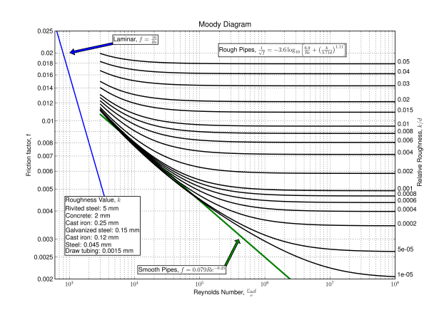
It should be noted that the correlation for “Smooth Pipes” is incorrect; for smooth pipes, it is best to assume that k = 0 using the “Rough Pipes” equation. If you don’t like this chart, use the one in your textbook.
1 The instructor’s handout has a worked example of how this is done.

I enjoyed readiing your post
LikeLike