
Channeling fluid flow through pipes is an everyday occurrence. We see it in plumbing, industrial plants, and fluid power (hydraulic) systems. A proper understanding of the basics of fluid flow in pipes–including measurement and losses–is essential for proper configuration of these systems. In this monograph we’ll concentrate on incompressible fluids; compressibility introduces some complications.
Classical Flow Metering: Theory
Euler’s inviscid equation states that
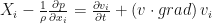
The fact that it is inviscid is important; we will see why shortly.
Slater and Frank (1947) show that this can be transformed to Bernoulli’s Equation, thus
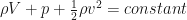
or, for passage from State 1 to State 2,

Bernoulli’s Equation is basically an expression of conservation of energy. There are three terms on each side:
- The first term is the energy from an external force field. For practical applications, this means gravity.
- The second is the pressure energy.
- The third is the velocity energy. We use
for velocity as a borrowing from CFD,
being the velocity in the y-direction. We’ll stick with one-dimensional flow in this case.
For our purposes we will ignore the external force field/gravity term. Leaving out the gravity term, Bernoulli’s Equation can be written thus:

where 

Let us now add the assumption that the fluid is incompressible, thus

Dividing through by the density yields

At this point the business about being inviscid comes into play; both Euler’s and Bernoulli’s Equations assume no energy losses due to viscosity. We could try something really fancy (like starting with the Navier-Stokes equations, which were actually first formulated by Saint-Venant) or we could do something simplistic like add a head (energy per unit mass) loss, like this:

Note that we have also divided through by the acceleration due to gravity 

Rearranging terms yields

Now let us turn to continuity of mass flow, which (unless a leak is sprung somewhere) is not subject to loss, or

Since the fluid is incompressible, the densities cancel out. At this point we also make another simplifying assumption: the velocity of the fluid across the cross-section of the pipe or restriction is uniform, or at least that the variation across the cross-section is not significant. Solving for 

Substituting this into the last form of Bernoulli’s Equation yields

If we are reading a U-tube manometer, the difference in column heights will be

Substituting this bring us to
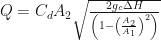
Assuming the uniform flow across the cross-section, the flow rate is

Substituting and solving for the flow rate, we have at last
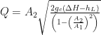
Up to now, it probably seems that we’ve pulled several “rabbits out of a hat.” These are simplifying assumptions that are based on experimental experience, the physical reality of the experiment, or both. But we have saved the biggest rabbit for last: we will dispense with the head loss term 


Classical Flow Metering: Implementation
Now that we have all of this theory, we ask ourselves, “What’s it good for?” There are two ways we can take this; the first thing we’ll consider is flow measurement. In short, we can set up a place in the flow where we change the flow area and, by measuring the pressure difference, we can determine the flow. This is the way flow has been measured in pipes for many years.
Let’s consider a couple of examples. The first is a sharp-edged orifice, simply a plate placed in the flow stream as shown below.

Here we see a U-tube manometer which measures pressure on the upstream and downstream side of the orifice. The fluid velocity varies as we have shown. The placement of the orifices is an important problem in using this type of device.
The major problem with this type of orifice is that it will measure fluid flow, but generates significant losses in use. A more efficient measuring device from that standpoint is the venturi meter, shown below.

The setup is similar except for the (God forbid) mercury manometer, which worked but, because of its hazards, is mercifully rare. The practical drawback to a venturi flowmeter is the long pipe length it occupies, which can be difficult to include in a busy piping system.
The efficiency variation can be seen in the coefficients of discharge, which vary from around 0.6 for a sharp-edged orifice to just under unity for a venturi meter. There are also flow meters which occupy a middle ground between the two, such as the rounded edge manometer.
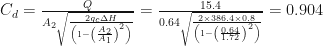
One might calibrate a flow meter by measuring its discharge coefficient 
As an example, consider a venturi where the inlet pipe diameter is 1.48″ and the throat diameter is 0.9″. A water flow of 4 gallons/minute (GPM) flow through the venturi at room temperature. The water manometer shows a head differential of 0.8″. What is the discharge coefficient?
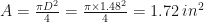
First, we do some preliminary conversions. The cross-sectional area of the venturi inlet pipe is 1.72 sq.in. and of the throat 0.64 sq.in. The flow in the inlet pipe is

Note that we’re using inches instead of feet. For problems of this scale, it’s really more convenient, even though it’s not really a “proper” way to do it. This means that 
We said we’d like to compute the Reynolds number for this discharge coefficient. Reynolds number is

The diameter for this case is the inlet diameter, as noted in Getting the Reynolds Number Right. We need first to compute the average velocity, which is

Using the value of kinematic viscosity given in Variation in Viscosity and inserting the appropriate unit conversions yields
Other Flow Meters
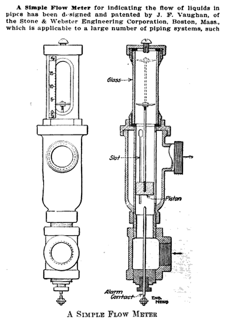
As flow meters go, classical flow meters are not as common as they used to be to measure flow. We think of other methods as “new” but the Rotameter was first patented in 1908. At the right is a variation of the concept dating from 1914. Rotameters are still very commonly used, although their accuracy can be highly variable. Today we have devices such as paddle wheel and magnetic flowmeters to more accurately measure the flow and to report the results to computer controlled systems.
“Minor” Losses in Systems
Another important application of this theory is the prediction of “minor” losses in such restrictions as valves, elbows, enlargements or contractions in the piping and other flow constrictions in the system. The use of the term “minor” is misleading; careless design can turn these into major losses very quickly, and the designer must be diligent in avoiding them if he or she wants a successful design. (Unless, of course, you’re trying to restrict fluid flow…)
Picking up where we left off in the theory, dividing both sides by the small area yields

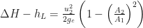
Eliminating the square root,

Solving for the head differential,

Since we normally prefer to consider the velocity in the incoming pipe

and then

We normally prefer to determine the second fraction on the right hand side experimentally as a loss or resistance coefficient 

The derivation indicates that, unlike the discharge coefficient, the loss or resistance coefficient can and frequently does exceed unity. It is obviously possible to use this equation to determine

As an example, consider a gate valve with an inlet diameter of 1.48″. Water is flowing through this and the manometer is likewise a water manometer. For a measured through flow of 15.9 gallons per minute, the manometer reads a differential height of 1.3″. What is the K value of the gate valve at this position and flow?
First, we compute the cross-sectional area of the inlet pipe (the customary “reference area” in this case.) That of course is
The flow must be converted as follows

The average velocity is thus the flow divided by the area, or

Since 
Flow in Pipes and the Moody Chart
It may seem like the long way around, but with the topic of flow metering and “minor” losses out of the way, we now consider the issue of losses in pipes. For straight pipes, the “classic” implementation of this is the Moody Chart, first published around World War II. One of these is shown below (from this site):
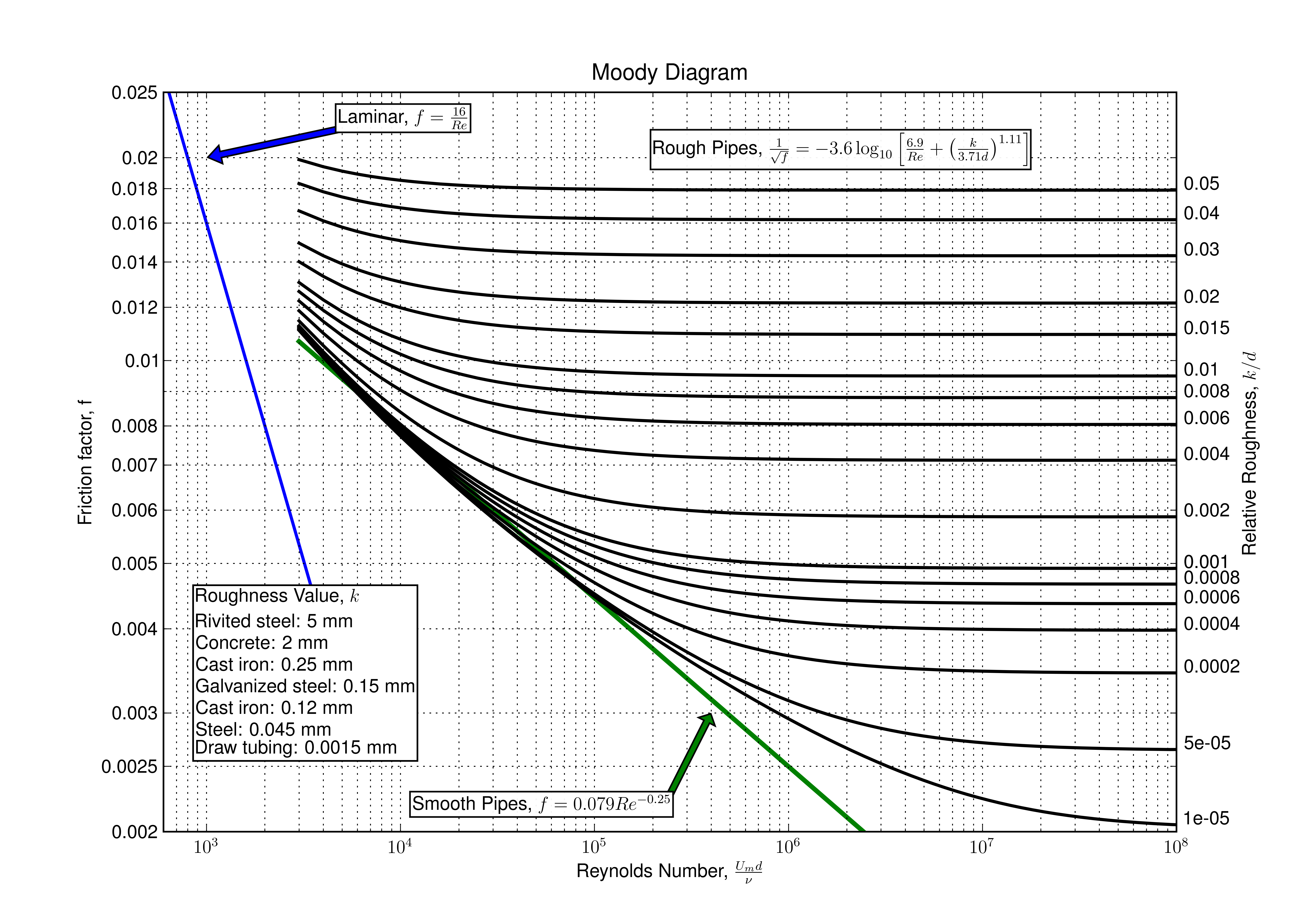
Note that the roughness values 
Although the chart can be used “as is” correlations have been developed, which are certainly more convenient in a spreadsheet than the chart. Some of those are shown on the chart above. The correlation for “Smooth Pipes” should not be used at all, and an inspection of the way the green line is drawn will show why this is so. The correlation for “Rough Pipes” can be improved on; a correlation to do that (good for turbulent flow in the range 
![f = \frac{1}{4\left[ log\left( \frac{\epsilon}{3.7 D}+\frac{5.74}{R_e^{0.9}} \right) \right]^2}](https://s0.wp.com/latex.php?latex=f+%3D+%5Cfrac%7B1%7D%7B4%5Cleft%5B+log%5Cleft%28+%5Cfrac%7B%5Cepsilon%7D%7B3.7+D%7D%2B%5Cfrac%7B5.74%7D%7BR_e%5E%7B0.9%7D%7D+%5Cright%29+%5Cright%5D%5E2%7D+&bg=%23ffffff&fg=%23111111&s=0&c=20201002)
where 
A “quick and dirty” replacement for the “Smooth Pipes” correlation for turbulent flow is

As an example, consider a 12 gpm flow of water at room temperature through a 12′ straight stretch of 1/2″ Type L copper tubing. What is the head loss we would expect?
The first thing we need to note is that Type L copper tubing has an I.D. of 0.545″ = 0.0452′. Again Mott (1994) gives typical values of roughness for this type of tubing as 

The head loss (the ordinate on the Moody Chart) we would expect is given as follows:

The Reynolds number (the abscissa on the Moody Chart) is given earlier, and the reader is exhorted to review Getting the Reynolds Number Right.
One thing we can do to make things a little simpler (this from Streeter (1966)) is to rewrite both formulas to allow direct input of the flow. Doing this yields

and

It is important that the units of flow are consistent with the rest of the units. Since we’re going to be doing this in feet, 
Knowing the Reynolds Number and the relative roughness, we can proceed. The Reynolds number (with properties of water from Variation in Viscosity) is

This is in the turbulent range; we can use the formula above. The friction factor is thus
![f = \frac{1}{4\left[ log\left( \frac{0.000005}{3.7\,0.0452}+\frac{5.74}{68910^{0.9}} \right) \right]^2} = 0.0199](https://s0.wp.com/latex.php?latex=f+%3D+%5Cfrac%7B1%7D%7B4%5Cleft%5B+log%5Cleft%28+%5Cfrac%7B0.000005%7D%7B3.7%5C%2C0.0452%7D%2B%5Cfrac%7B5.74%7D%7B68910%5E%7B0.9%7D%7D+%5Cright%29+%5Cright%5D%5E2%7D+%3D+0.0199&bg=%23ffffff&fg=%23111111&s=0&c=20201002)
Comparison with the Moody Chart should show that this is very close.
The head loss is thus

The inches conversion is done because most manometers–physical and digital–measure water head differences in inches.
Equivalent Length
We can combine our work on both minor losses and pipe losses by considering the concept of equivalent length of pipe. Thus, we can say that, for a given diameter of pipe, a restriction has the same effect on the pressure drop of a system as a certain length of pipe 

The friction factor 
Equivalent length is a good practical way of looking at the losses in a section of pipe with all of its restrictions without getting into “apples and oranges” comparisons. Since they are in series, the equivalent and actual lengths of the pipe are simply added.
Conclusion
Losses in fluid elements such as valves and pipes can be considered in two ways. Orifices such as the sharp-edged orifice and the venturi can be used to measure the flow in the system. The theory can be flipped to enable us to estimate losses in the system and thus avoid unwanted energy, pressure and flow degradation of the fluid system.
