An Overview of Stokes’ Law

Free Body Diagram of Sphere Falling Through a Viscous Fluid (modified from Strelkov)

Stokes’ Law (named after the British scientist G.G. Stokes, who came up with the law in 1851) is an important combination of fluid and solid mechanics and finds use in a number of applications. In addition to being a good example of “static” (in this case constant velocity) equilibrium it also touches on two other important topics in fluid mechanics: Buoyancy and Stability and Lift and Drag of bodies through a fluid. The presentation here is taken from Strelkov’s Mechanics with modifications.

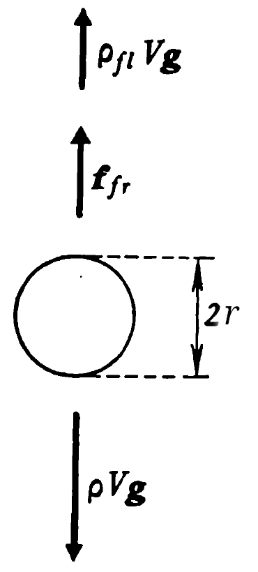
Consider a sphere falling through a viscous fluid. The free body diagram is shown on the right. There are three forces on the ball, from top to bottom:

Buoyant force of the water on the ball. As noted in Buoyancy and Stability, it’s possible to compute this by computing the differential pressure between the top and the bottom of the ball, but it’s a lot easier to apply Archimedes’ Law directly.
Viscous force of the fluid on the ball. Since we’re assuming the ball is falling, the viscous force opposes the motion of the ball.
Force of gravity on the ball, or its weight.

Variables are as follows:

ρ_fl = density of the fluid
f_fr = viscous force on the fluid
f_g = force of gravity on the ball
f_b = buoyant force on the ball
V = volume of the sphere
g = acceleration due to gravity
r = radius of the sphere
ρ = density of the ball
m = mass of the ball

The equation of motion (from Dynamics) is as follows:

m{\frac {d^{2}}{d{t}^{2}}}x(t)=f_{{g}}-f_{{b}}-f_{{{\it fr}}}

The three forces on the right hand side are defined as follows:

f_g = V\rho\,{\it g}

f_b = V\rho_{{{\it fl}}}{\it g}

f_{fr} = 6\,\pi \,\mu\,r{\frac {d}{dt}}x(t)

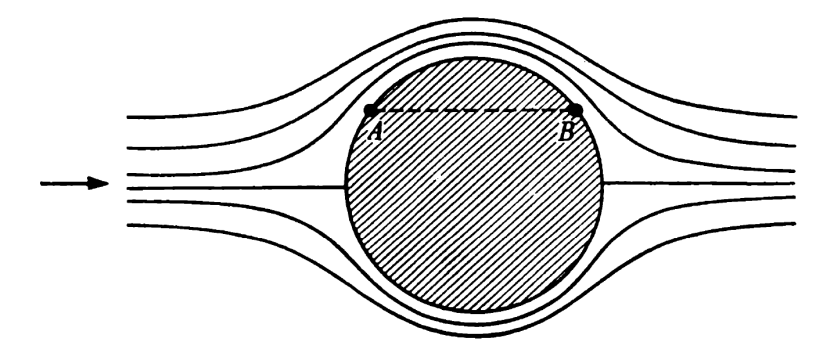
The last assumes that the flow is laminar and intertial forces in the fluid are not considered. An example of laminar flow is shown below. More discussion on flow around spheres in general is give in Fluid Mechanics Laboratory Video: Wind Tunnel Testing.

Laminar Flow Around a Sphere or Cylinder (from Strelkov)

Substituting into the equation of motion yields

m{\frac {d^{2}}{d{t}^{2}}}x(t)=V\rho\,{\it g}-V\rho_{{{\it fl}}}{\it g}-6\,\pi \,\mu\,r{\frac {d}{dt}}x(t)

Noting that the volume of a sphere is

V = 4/3\,\pi \,{r}^{3}

and also noting that the mass of the sphere is its volume times its density, substituting yields

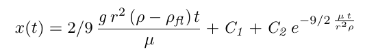
4/3\,\rho\,\pi \,{r}^{3}{\frac {d^{2}}{d{t}^{2}}}x(t)=4/3\,\pi \,{r}^{ 3}\rho\,{\it g}-4/3\,\pi \,{r}^{3}\rho_{{{\it fl}}}{\it g}-6\,\pi \, \mu\,r{\frac {d}{dt}}x(t)

The solution of this equation is

Taking the time derivative of this yields

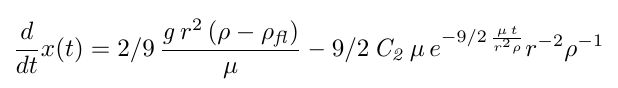
At this point we could go on and determine the constants of integration, but our interest is to determine the velocity of the ball at a large value of time (its “terminal velocity.”) We note that the second term on the right hand side vanishes as t approaches infinity, and so this terminal velocity is

v_{0}=2/9\,{\frac{{\it g}\,{r}^{2}\left(\rho-\rho_{{\it fl}}\right)}{\mu}}

Stokes’ Law has a number of applications. One of them is to use a falling sphere in a viscometer; solving the last equation for viscosity allows us to estimate the viscosity of a fluid when the parameters of the ball and the terminal velocity is known. Another, more complicated application is the hydrometer test in soil mechanics, where the falling of soil particles is used to determine the particle size distribution for very small particles.

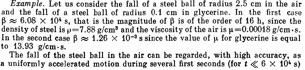
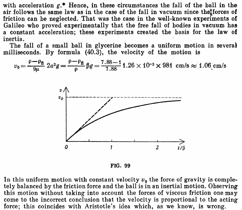
An example of this is given below, from Strelkov. Note that (he also uses a for radius)