Computing Open Channel Flow Using a Pitot Tube

In our last post we discussed the basics of hydraulic jump. We showed how the flow across the jump could be estimated using the depths of the water before and after the jump. In this post we will show another method, using a pitot tube, which is also used in a wide variety of other applications.

The calculations in our earlier post assumed the velocity of the water to be uniform. In a flow channel with parallel straight sides and rectangular cross-section, we assumed the flow to be

$Q = uwy$ (1)

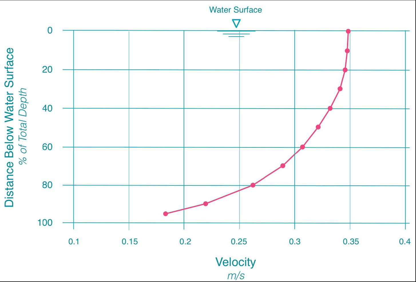
where the variables are as before. For both open and closed channels, however, the velocity will not be uniform; the velocity we used was an average velocity. If we actually measured the velocity at various points in the flow, we would get different results for different places, as illustrated below (from Open Channel Flow Measurement):

The following presentation assumes a rectangular cross-section with parallel walls.

Pitot Tube Measurements

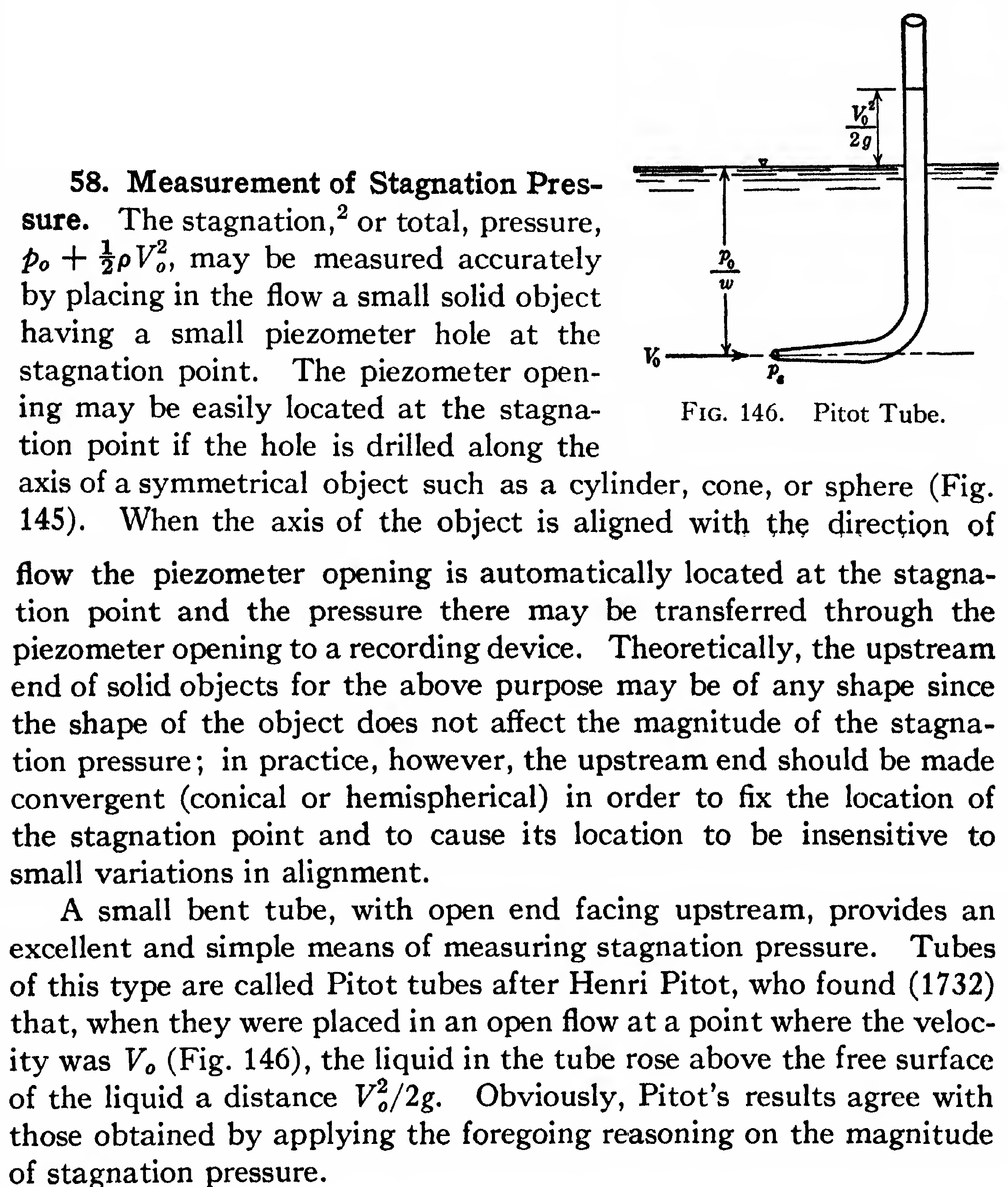
We discussed the concept behind the Pitot tube in Wind Tunnel Testing. The simplest way to show this for open channel flow is to use the presentation of Vennard (1940):

A more formal presentation with Bernoulli’s Equation follows. That equation is

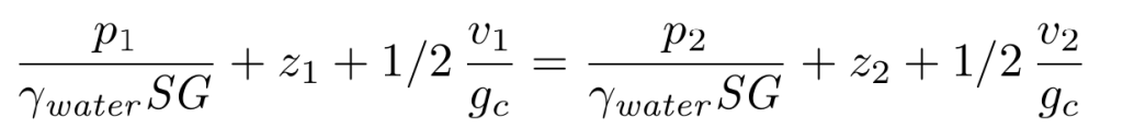
(2)

where

p₁, p₂ = static pressures at Points 1 and 2
z₁, z₂ = elevations at Points 1 and 2
γ_water = unit weight of water
SG = specific gravity of fluid in question
g_c = acceleration due to gravity

We then make the following definitions and substitutions:

We define the control volume: Point 1 is at the tip of the Pitot tube immersed in the water, Point 2 is the surface of the water column which is above the main surface of the water.
We define the datum as the main surface of the water. This means that z₁ is the distance from the main surface down to Point 1 (negative) and z₂ is the distance from the main surface up to the surface in the tube (positive.)
The static pressure at Point 1 is the depth of the fluid times the distance from the main free surface of the water, or $-z_1 \times \gamma_{water} \times SG$ . The minus sign is necessary since z₁ is negative and the static pressure is positive.
The static pressure p₂ and velocity v₂ at Point 2 are zero.

Applying these definitions and substitutions to Equation (2) yields

z_{{2}}=1/2\,{\frac {v_{1}^2}{g_{{c}}}}

(3)

which agrees with the narrative above.

Integrating the Results

Separating the static pressure from the stagnation (dynamic) pressure is fairly simple in open channel flow, although reading the results can be tricky if the flow level varies. We thus take several measurements at several heights and compute a velocity at each point, getting a velocity profile for the flow. But how to integrate this relationship for a total flow? There are several methods.

One would be to take a trend line of the results (as discussed in Least Squares Analysis and Curve Fitting) and integrate it in closed form. For this to work requires that the trend line have a very good correlation with the original data.

Another would be to take the results and graphically integrate them. For many engineering applications, graphical methods were popular for many years because they avoided many difficult calculations which strained the limited computational power of the time. Although the results were approximate, with CAD a higher degree of precision can be obtained than was possible before. The tricky part of a graphical method such as this is the scaling, which must be understood to properly interpret the results.

Yet another is the use of numerical integration, generally piecewise with methods such as the Trapezoidal Rule and Simpson’s Rule. With a properly laid out spreadsheet, this can be done with minimal effort, although attention to detail is crucial to success.

An implementation of numerical integration can be used which simplifies the calculations, and is suggested in Open Channel Flow Measurement. It involves a little pre-planning in that the points where the data is taken need to be pre-determined (they should be in any case.) Since the more points of data the more accurate the result (all other things equal,) we’ll use six points. Those points are at the surface, at the bottom of the channel, and at 20% (0.2), 40% (0.4), 60% (0.6) and 80% (0.8) of the total depth. The mean velocity can be thus computed as follows:

$u_{mean}=\frac{u_{surface}+0.2u_{0.2}+0.2u_{0.4}+0.2u_{0.6}+0.2u_{0.8}+u_{bottom}}{10}$

Boundary layer considerations would indicate that the velocity at the bottom of the channel be zero, but if it is possible to take a measurement it would be better.

Once the $u_{mean}$ is calculated, it can be used in the equation at the beginning of the post to estimate the flow in the channel.

References

Vennard, J.K. (1940) Elementary Fluid Mechanics. New York: John Wiley & Sons, Inc.